<?xml version="1.0" encoding="utf-8"?><feed xmlns="http://www.w3.org/2005/Atom" ><generator uri="https://jekyllrb.com/" version="3.10.0">Jekyll</generator><link href="https://rajeshphy.github.io/feed.xml" rel="self" type="application/atom+xml" /><link href="https://rajeshphy.github.io/" rel="alternate" type="text/html" /><updated>2026-06-13T16:58:30+00:00</updated><id>https://rajeshphy.github.io/feed.xml</id><title type="html">Rajesh Kumar</title><subtitle>Lecture Notes</subtitle><author><name>Rajesh Kumar</name></author><entry><title type="html">Paper I Exam Template</title><link href="https://rajeshphy.github.io/exam-paper-i-template/" rel="alternate" type="text/html" title="Paper I Exam Template" /><published>2026-06-12T19:18:00+00:00</published><updated>2026-06-12T19:18:00+00:00</updated><id>https://rajeshphy.github.io/exam-paper-i-template</id><content type="html" xml:base="https://rajeshphy.github.io/exam-paper-i-template/"><![CDATA[<p>Use this page for Paper I material.</p>

<h2 id="notice">Notice</h2>

<ul>
  <li>Add Paper I instructions.</li>
  <li>Add language, syllabus, and schedule details.</li>
</ul>

<h2 id="study-material">Study Material</h2>

<table>
  <thead>
    <tr>
      <th>Section</th>
      <th>File</th>
    </tr>
  </thead>
  <tbody>
    <tr>
      <td>Hindi</td>
      <td>Add link</td>
    </tr>
    <tr>
      <td>English</td>
      <td>Add link</td>
    </tr>
    <tr>
      <td>General teaching aptitude</td>
      <td>Add link</td>
    </tr>
  </tbody>
</table>]]></content><author><name>Rajesh Kumar</name></author><category term="exam" /><category term="exam" /><category term="paper-i" /><category term="template" /><summary type="html"><![CDATA[Use this page for Paper I material.]]></summary></entry><entry><title type="html">Physical Science Exam Template</title><link href="https://rajeshphy.github.io/exam-physical-science-template/" rel="alternate" type="text/html" title="Physical Science Exam Template" /><published>2026-06-12T19:17:00+00:00</published><updated>2026-06-12T19:17:00+00:00</updated><id>https://rajeshphy.github.io/exam-physical-science-template</id><content type="html" xml:base="https://rajeshphy.github.io/exam-physical-science-template/"><![CDATA[<p>Use this page for Physical Science exam preparation.</p>

<h2 id="notice">Notice</h2>

<ul>
  <li>Add exam schedule updates.</li>
  <li>Add syllabus and important instructions.</li>
</ul>

<h2 id="preparation-material">Preparation Material</h2>

<table>
  <thead>
    <tr>
      <th>Area</th>
      <th>File</th>
    </tr>
  </thead>
  <tbody>
    <tr>
      <td>Mathematical physics</td>
      <td>Add link</td>
    </tr>
    <tr>
      <td>Classical mechanics</td>
      <td>Add link</td>
    </tr>
    <tr>
      <td>Quantum mechanics</td>
      <td>Add link</td>
    </tr>
  </tbody>
</table>]]></content><author><name>Rajesh Kumar</name></author><category term="exam" /><category term="exam" /><category term="physical-science" /><category term="template" /><summary type="html"><![CDATA[Use this page for Physical Science exam preparation.]]></summary></entry><entry><title type="html">Magnetic Oscillator Complexity</title><link href="https://rajeshphy.github.io/magnetic-oscillator-complexity/" rel="alternate" type="text/html" title="Magnetic Oscillator Complexity" /><published>2026-05-31T16:30:00+00:00</published><updated>2026-05-31T16:30:00+00:00</updated><id>https://rajeshphy.github.io/Magnetic-Oscillator</id><content type="html" xml:base="https://rajeshphy.github.io/magnetic-oscillator-complexity/"><![CDATA[<p>A charged harmonic oscillator in an external magnetic field appears to be a simple quantum-mechanical system, yet it provides a clean setting for understanding quantum complexity in thermal states. The central question is how a magnetic field modifies the difficulty of constructing a thermal quantum state from a simple reference state. In the work of Avramov, Radomirov, Rashkov, and Vetsov, this question is addressed by combining the dynamics of a charged oscillator, the thermofield-double construction, Gaussian-state covariance matrices, and Nielsen’s geometric notion of circuit complexity.</p>

<h2 id="from-magnetic-oscillator-to-two-effective-frequencies">From Magnetic Oscillator to Two Effective Frequencies</h2>

<p>Quantum complexity entered physics because entanglement entropy alone does not always capture the continued evolution of quantum states. In holographic systems, for example, the interior geometry of certain black holes keeps evolving even after entanglement entropy has saturated. Complexity therefore asks a different question: not how entangled a state is, but how difficult it is to construct.</p>

<p>In Nielsen’s geometric approach, one begins with a simple reference state $|\psi_R\rangle$ and constructs a target state $|\psi_T\rangle$ by applying elementary quantum operations. Rather than counting gates directly, one studies all possible paths from the reference state to the target state and assigns a cost to each path. The complexity is the length of the shortest such path.</p>

<p>The harmonic oscillator is a natural testing ground because many physical systems reduce to oscillator modes near equilibrium, including molecular vibrations, lattice vibrations, electromagnetic field modes, quantum fields, trapped ions, and superconducting circuits.</p>

<p>Consider a charged particle in a two-dimensional harmonic trap. Without a magnetic field, the Hamiltonian is</p>

\[H=\frac{p_x^2+p_y^2}{2m}+\frac{1}{2}m\omega_0^2(x^2+y^2).\]

<p>In this case, the particle behaves like an ordinary two-dimensional harmonic oscillator whose motion is governed solely by the restoring force of the harmonic potential. The frequency of oscillation is $\omega_0$, and clockwise and anticlockwise motions are energetically equivalent.</p>

<p>When a magnetic field is applied along the $z$-direction, the canonical momentum is replaced by</p>

\[\mathbf{p}\rightarrow \mathbf{p}-e\mathbf{A},\]

<p>where $\mathbf{A}$ is the vector potential associated with the magnetic field.</p>

<div style="border:2px solid #b91c1c; background:#fff5f5; padding:1rem; border-radius:8px; margin:1.25rem 0;">
  <strong style="display:block; color:#7f1d1d; font-size:1.05rem; margin-bottom:0.6rem;">Why Is the Symmetric Gauge Used?</strong>

  <p>The magnetic field $\mathbf B$ is the physical quantity, while the vector potential $\mathbf A$ is not unique. Any vector potential satisfying</p>

  $$
  \mathbf B=\nabla\times\mathbf A
  $$

  <p>produces the same magnetic field. For a uniform magnetic field along the $z$-direction,</p>

  $$
  \mathbf B=(0,0,B),
  $$

  <p>many choices of $\mathbf A$ are possible. For example the Landau gauge
    $$
    \mathbf A=
    \begin{pmatrix}
    0\\
    Bx\\
    0
    \end{pmatrix},
    $$
  is often used in condensed matter physics. However, the Landau gauge breaks the symmetry between the $x$ and $y$ coordinates, which can complicate the analysis of a rotationally symmetric system like the harmonic oscillator. In contrast, the symmetric gauge treats $x$ and $y$ on equal footing, preserving the rotational symmetry and making the role of angular momentum more transparent. 
  The authors use the <strong>symmetric gauge</strong></p>

  $$
  \mathbf A=
  \frac{B}{2}
  \begin{pmatrix}
  -y\\
  x\\
  0
  \end{pmatrix},
  $$

  <p>This choice makes the role of angular momentum explicit and greatly simplifies the analysis in polar coordinates.</p>
</div>

<p>Using this gauge, the kinetic term acquires additional contributions. After expanding</p>

\[(\mathbf p-e\mathbf A)^2,\]

<p>one obtains an extra interaction term</p>

\[-\frac{eB}{2m}(xp_y-yp_x).\]

<div style="border:2px solid #4a5568; padding:15px; border-radius:8px; background:#f8fafc;">

<strong>Expansion of $(\mathbf p-e\mathbf A)^2$</strong>

<p>
The square of a vector means a dot product with itself:
</p>

$$
(\mathbf p-e\mathbf A)^2
=
(\mathbf p-e\mathbf A)\cdot(\mathbf p-e\mathbf A).
$$

<p>
Using the symmetric gauge,
</p>

$$
\mathbf A
=
\frac{B}{2}
\begin{pmatrix}
-y\\
x
\end{pmatrix},
$$

<p>
we obtain
</p>

$$
\mathbf p-e\mathbf A
=
\begin{pmatrix}
p_x+\frac{eB}{2}y\\
p_y-\frac{eB}{2}x
\end{pmatrix}.
$$

<p>
Therefore,
</p>

$$
(\mathbf p-e\mathbf A)^2
=
\left(p_x+\frac{eB}{2}y\right)^2
+
\left(p_y-\frac{eB}{2}x\right)^2.
$$

<p>
Expanding,
</p>

$$
(\mathbf p-e\mathbf A)^2
=
p_x^2+p_y^2
+\frac{e^2B^2}{4}(x^2+y^2)
+\frac{eB}{2}(p_xy+yp_x)
-\frac{eB}{2}(p_yx+xp_y).
$$

<p>
Using
</p>

$$
[p_x,y]=0,
\qquad
[p_y,x]=0,
$$

<p>
gives
</p>

$$
p_xy=yp_x,
\qquad
p_yx=xp_y.
$$

<p>
Hence,
</p>

$$
(\mathbf p-e\mathbf A)^2
=
p_x^2+p_y^2
+\frac{e^2B^2}{4}(x^2+y^2)
-eB(xp_y-yp_x).
$$

<p>
Recognizing
</p>

$$
L_z=xp_y-yp_x,
$$

<p>
the final result becomes
</p>

$$
\boxed{
(\mathbf p-e\mathbf A)^2
=
p_x^2+p_y^2
+\frac{e^2B^2}{4}(x^2+y^2)
-eB\,L_z
}.
$$

<p>
Thus, the magnetic field contributes:
</p>

<ul>
  <li>$p_x^2+p_y^2$: ordinary kinetic energy,</li>
  <li>$\frac{e^2B^2}{4}(x^2+y^2)$: additional harmonic confinement,</li>
  <li>$-eB\,L_z$: coupling between the magnetic field and angular momentum.</li>
</ul>

</div>

<p>This shows that the magnetic field couples directly to the orbital angular momentum of the particle. Physically, the energy now depends on the sense of rotation. States rotating clockwise and anticlockwise are no longer equivalent because the magnetic field favors one direction of circulation over the other.</p>

<p>This effect has a simple classical interpretation. The harmonic trap continuously pulls the particle toward the origin, while the magnetic field generates a Lorentz force that bends the trajectory into circular motion. The resulting dynamics arise from a competition between these two tendencies: confinement by the harmonic potential and rotation induced by the magnetic field.</p>

<p>One of the most important consequences is that the original two-dimensional oscillator no longer behaves as a single oscillator. The angular-momentum coupling lifts the degeneracy between opposite rotational modes and splits the system into two independent normal modes with different frequencies. These frequencies will later appear as</p>

\[\omega_1=
\frac{\sqrt{4\omega_0^2+\omega_c^2}+\omega_c}{2},
\qquad
\omega_2=
\frac{\sqrt{4\omega_0^2+\omega_c^2}-\omega_c}{2},\]

<p>where</p>

\[\omega_c=\frac{eB}{m}\]

<p>is the cyclotron frequency. Thus, the magnetic field effectively transforms a single oscillator into two oscillators whose frequencies depend on the strength of the field.</p>

<p>After diagonalization, the Hamiltonian becomes equivalent to two independent oscillators:</p>

\[H=\hbar\omega_1\left(n+\frac{1}{2}\right)+\hbar\omega_2\left(k+\frac{1}{2}\right).\]

<p>The magnetic field therefore splits the original planar oscillator into two effective modes with frequencies</p>

\[\omega_1=\frac{\sqrt{4\omega_0^2+\omega_c^2}+\omega_c}{2},\]

<p>and</p>

\[\omega_2=\frac{\sqrt{4\omega_0^2+\omega_c^2}-\omega_c}{2}.\]

<p>Here</p>

\[\omega_c=\frac{eB}{m}\]

<p>is the cyclotron frequency. Thus, before complexity is even introduced, the main physical effect of the magnetic field is to convert one two-dimensional oscillator into two independent oscillators whose frequencies depend on $B$.</p>

<h2 id="thermal-states-tfd-construction-and-gaussian-covariance-geometry">Thermal States, TFD Construction, and Gaussian Covariance Geometry</h2>

<p>Complexity is most naturally defined for pure quantum states, but a system at temperature $T$ is described by the mixed thermal density matrix</p>

\[\rho=\frac{e^{-\beta H}}{Z},\]

<p>where</p>

\[\beta=\frac{1}{kT}.\]

<p>To apply pure-state methods to thermal physics, one uses the thermofield-double construction. The Hilbert space is doubled into left and right copies, and the thermal density matrix is represented through a pure entangled state:</p>

\[|TFD\rangle=\frac{1}{\sqrt{Z}}\sum_n e^{-\beta E_n/2}|n\rangle_L|n\rangle_R.\]

<p>Although the full thermofield-double state is pure, each subsystem separately behaves thermally. This allows the complexity of a thermal system to be studied using pure-state geometric tools.</p>

<p>For the magnetic oscillator, the diagonalized system contains two independent frequencies, so two squeezing parameters appear:</p>

\[\tanh\alpha_i=e^{-\beta\hbar\omega_i/2}.\]

<p>The parameters $\alpha_1$ and $\alpha_2$ measure the entanglement between the two copies of the system. At low temperature, $\beta\to\infty$, so</p>

\[e^{-\beta\hbar\omega_i/2}\to 0,\]

<p>and therefore</p>

\[\alpha_i\to 0.\]

<p>The thermofield-double state then approaches the vacuum-like reference state. At high temperature, $\beta\to 0$, so</p>

\[e^{-\beta\hbar\omega_i/2}\to 1,\]

<p>and the squeezing parameters become large. The state becomes strongly entangled, and its distance from the reference state increases.</p>

<p>The thermofield-double states in this problem are Gaussian states. For Gaussian states, the full state is completely determined by second moments such as</p>

\[\langle XX\rangle,\qquad \langle PP\rangle,\qquad \langle XP\rangle.\]

<p>These second moments are assembled into a covariance matrix $G$. Therefore, instead of tracking the full wavefunction, one can study the covariance matrix.</p>

<p>Complexity compares a reference state and a target state. If their covariance matrices are $G_R$ and $G_T$, the relative covariance matrix is</p>

\[\Delta=G_TG_R^{-1}.\]

<p>If the reference and target states coincide, then</p>

\[G_T=G_R,\]

<p>so</p>

\[\Delta=I,\]

<p>and no circuit is needed. Thus $\Delta$ measures the deformation required to transform the reference covariance geometry into the target covariance geometry.</p>

<p>For Gaussian states, the complexity is written as</p>

\[C=\frac{1}{2}\sqrt{\mathrm{Tr}\left(\ln\Delta\right)^2}.\]

<p>The logarithm extracts the generator of the transformation from the reference state to the target state, and the trace of its square gives a natural geometric length. Hence this formula is the covariance-matrix version of the shortest-path distance in Nielsen’s complexity geometry.</p>

<h2 id="magnetic-field-temperature-and-complexity-dynamics">Magnetic Field, Temperature, and Complexity Dynamics</h2>

<p>The thermofield-double state evolves in time through the Hamiltonian. Since the diagonalized Hamiltonian contains two frequencies, $\omega_1$ and $\omega_2$, the covariance matrix develops oscillatory terms such as</p>

\[\cos(\omega_i t),\]

<p>and</p>

\[\sin(\omega_i t).\]

<p>Consequently, the complexity becomes time-dependent and oscillatory.</p>

<p>In the strong magnetic-field regime,</p>

\[\omega_c\gg\omega_0,\]

<p>the two effective frequencies separate strongly:</p>

\[\omega_1\gg\omega_2.\]

<p>The fast mode oscillates rapidly, while the slow mode controls the broad structure of the complexity curve. The resulting behaviour is nearly periodic, with an approximate period</p>

\[T\approx\frac{\pi}{\omega_2}.\]

<p>Thus a strong magnetic field produces relatively regular complexity oscillations.</p>

<p>In the weak magnetic-field regime,</p>

\[\omega_c\ll\omega_0,\]

<p>the two frequencies become nearly equal:</p>

\[\omega_1\approx\omega_2.\]

<p>When two nearly equal frequencies are superposed, beating appears. The same mechanism occurs in the complexity: the oscillations alternate between regions of large and small amplitude. The beating period is approximately</p>

\[T\approx\frac{\pi}{\omega_1-\omega_2}.\]

<p>Temperature affects complexity through the squeezing relation</p>

\[\tanh\alpha_i=e^{-\beta\hbar\omega_i/2}.\]

<p>As temperature increases, $\beta$ decreases, and the squeezing parameters $\alpha_i$ increase. Larger squeezing means stronger left-right entanglement in the thermofield-double state and a larger geometric separation from the reference state. Therefore, complexity increases with temperature. In the low-temperature limit it approaches a minimum value, while in the high-temperature limit it becomes unbounded.</p>

<h2 id="lloyd-bound-and-central-physical-message">Lloyd Bound and Central Physical Message</h2>

<p>A natural question is whether complexity can grow arbitrarily fast. Lloyd’s bound proposes that the rate of complexity growth is limited by the available energy:</p>

\[|\dot{C}|\leq \frac{2U}{\pi\hbar}.\]

<p>Here $U$ is the internal energy. The physical idea is that energy limits the maximum rate at which a system can perform computation, so complexity growth cannot exceed an energy-controlled bound.</p>

<p>The authors compare the maximum complexity growth rate with Lloyd’s bound by computing both $|\dot{C}|_{\max}$ and the internal energy $U$. They find that, for the magnetic oscillator system,</p>

\[|\dot{C}|_{\max}&lt;\frac{2U}{\pi\hbar}.\]

<p>Thus the charged harmonic oscillator in a magnetic field respects Lloyd’s bound across the parameter regimes considered.</p>

<p>The central message is that a charged harmonic oscillator in a magnetic field effectively becomes two independent oscillators with magnetic-field-dependent frequencies. These frequencies determine the thermofield-double state, the squeezing parameters, the covariance matrix, and ultimately the quantum complexity. Strong magnetic fields produce regular oscillatory complexity, weak magnetic fields generate beating patterns, higher temperature increases complexity, and the rate of complexity growth remains below Lloyd’s energy bound.</p>]]></content><author><name>Rajesh Kumar</name></author><category term="research" /><category term="quantum-complexity" /><category term="harmonic-oscillator" /><category term="magnetic-field" /><summary type="html"><![CDATA[A charged harmonic oscillator in an external magnetic field appears to be a simple quantum-mechanical system, yet it provides a clean setting for understanding quantum complexity in thermal states. The central question is how a magnetic field modifies the difficulty of constructing a thermal quantum state from a simple reference state. In the work of Avramov, Radomirov, Rashkov, and Vetsov, this question is addressed by combining the dynamics of a charged oscillator, the thermofield-double construction, Gaussian-state covariance matrices, and Nielsen’s geometric notion of circuit complexity.]]></summary></entry><entry><title type="html">Shape Invariance and Ramos</title><link href="https://rajeshphy.github.io/shape-invariance/" rel="alternate" type="text/html" title="Shape Invariance and Ramos" /><published>2026-05-30T06:20:00+00:00</published><updated>2026-05-30T06:20:00+00:00</updated><id>https://rajeshphy.github.io/Shape-Invariance</id><content type="html" xml:base="https://rajeshphy.github.io/shape-invariance/"><![CDATA[<p>Shape invariance is one of the central algebraic mechanisms behind exactly solvable quantum potentials in supersymmetric quantum mechanics. Instead of solving the Schrödinger equation separately for each bound state, one factorizes the Hamiltonian, constructs partner potentials, and uses a parameter-shift rule to generate the entire spectrum recursively. Ramos’ contribution extends this classical idea to systems with several translated parameters by introducing translation-invariant combinations into the superpotential.</p>

<h2 id="from-schrödinger-equation-to-shape-invariance">From Schrödinger Equation to Shape Invariance</h2>

<p>In ordinary one-dimensional quantum mechanics, the bound-state problem begins with the eigenvalue equation</p>

\[H\psi_n(x)=E_n\psi_n(x),\]

<p>where</p>

\[H=-\frac{d^2}{dx^2}+V(x).\]

<p>Thus one must solve</p>

\[\left[-\frac{d^2}{dx^2}+V(x)\right]\psi(x)=E\psi(x).\]

<p>For most potentials, this second-order differential equation cannot be solved exactly. Supersymmetric quantum mechanics begins with a different question: can the Hamiltonian be written as a product of first-order differential operators?</p>

<p>Define</p>

\[A=\frac{d}{dx}+W(x),\]

<p>and</p>

\[A^\dagger=-\frac{d}{dx}+W(x),\]

<p>where $W(x)$ is called the superpotential. It is not the physical potential itself; rather, it is a generating function from which two partner potentials are constructed.</p>

<p>The two SUSY partner Hamiltonians are</p>

\[H_-=A^\dagger A,\]

<p>and</p>

\[H_+=AA^\dagger.\]

<p>Expanding them gives</p>

\[H_-=-\frac{d^2}{dx^2}+W^2(x)-W'(x),\]

<p>and</p>

\[H_+=-\frac{d^2}{dx^2}+W^2(x)+W'(x).\]

<p>Hence the partner potentials are</p>

\[V_-(x)=W^2(x)-W'(x),\]

<p>and</p>

\[V_+(x)=W^2(x)+W'(x).\]

<p>The two potentials differ only in the sign of the derivative term $W’(x)$. This partner structure becomes powerful when the superpotential also depends on a parameter $a$:</p>

\[W=W(x;a).\]

<p>Then</p>

\[V_-(x;a)=W^2(x;a)-W'(x;a),\]

<p>and</p>

\[V_+(x;a)=W^2(x;a)+W'(x;a).\]

<p>Shape invariance means that $V_+(x;a_0)$ has the same functional form as $V_-(x;a_1)$, except for an additive constant independent of $x$:</p>

\[V_+(x;a_0)=V_-(x;a_1)+R(a_0),\]

<p>where</p>

\[a_1=f(a_0).\]

<p>For many exactly solvable potentials, the shift is translational:</p>

\[a_1=a_0-1.\]

<p>Thus the condition becomes</p>

\[V_+(x;a)=V_-(x;a-1)+R(a).\]

<p>The crucial point is that the remainder $R(a)$ may depend on the parameter, but not on position. Therefore, the shape of the potential is preserved while the parameter changes. This converts the problem from differential-equation solving into algebraic parameter recursion:</p>

\[\text{Differential equation problem}\longrightarrow\text{algebraic parameter recursion}.\]

<h2 id="spectrum-ground-state-and-examples">Spectrum, Ground State, and Examples</h2>

<p>Once shape invariance holds, the energy spectrum follows from a ladder of shifted parameters. Let</p>

\[a_0=a.\]

<p>For translational shape invariance,</p>

\[a_1=a_0-1,\]

\[a_2=a_0-2,\]

<p>and in general</p>

\[a_k=a_0-k.\]

<p>The excited-state energies of $H_-$ are obtained by summing the remainders along this ladder:</p>

\[E_n=\sum_{k=1}^{n}R(a_k).\]

<p>This is the central algebraic result of shape invariance. The spectrum is built step by step from constants rather than by repeatedly solving the Schrödinger equation.</p>

<p>The ground state is even simpler. Since</p>

\[H_-=A^\dagger A,\]

<p>the lowest state satisfies</p>

\[A\psi_0=0.\]

<p>Using</p>

\[A=\frac{d}{dx}+W(x),\]

<p>we get</p>

\[\left(\frac{d}{dx}+W(x)\right)\psi_0(x)=0.\]

<p>Therefore,</p>

\[\frac{d\psi_0}{dx}=-W(x)\psi_0,\]

<p>and hence</p>

\[\frac{d}{dx}\ln\psi_0(x)=-W(x).\]

<p>After integration,</p>

\[\psi_0(x)=N\exp\left[-\int W(x)\,dx\right],\]

<p>where $N$ is a normalization constant. Thus the ground-state wavefunction is determined directly from the superpotential.</p>

<p>The excited states are obtained by applying raising operators with successively shifted parameters:</p>

\[\psi_n(x;a_0)\propto A^\dagger(a_0)A^\dagger(a_1)\cdots A^\dagger(a_{n-1})\psi_0(x;a_n).\]

<p>This formula shows that shape-invariant ladder construction is not simply repeated application of one fixed operator. The operator changes as the parameter shifts:</p>

\[a_0\to a_1\to a_2\to\cdots\to a_n.\]

<p>For the harmonic oscillator, choose</p>

\[W(x)=x.\]

<p>Then</p>

\[W^2(x)=x^2,\]

<p>and</p>

\[W'(x)=1.\]

<p>Hence</p>

\[V_-(x)=x^2-1,\]

<p>and</p>

\[V_+(x)=x^2+1.\]

<p>Thus</p>

\[V_+(x)=V_-(x)+2,\]

<p>so the remainder is</p>

\[R=2.\]

<p>The energy levels are therefore</p>

\[E_n=\sum_{k=1}^{n}2=2n.\]

<p>The ground state follows from</p>

\[\left(\frac{d}{dx}+x\right)\psi_0=0,\]

<p>giving</p>

\[\psi_0(x)=Ne^{-x^2/2}.\]

<p>For a Morse-type system, take</p>

\[W(x;a)=a-e^{-x}.\]

<p>The parameter ladder is</p>

\[a_k=a-k.\]

<p>With the corresponding remainder</p>

\[R(a_k)=2(a-k)-1,\]

<p>the energy is</p>

\[E_n=\sum_{k=1}^{n}\left[2(a-k)-1\right].\]

<p>That is,</p>

\[E_n=\sum_{k=1}^{n}(2a-2k-1).\]

<p>Using</p>

\[\sum_{k=1}^{n}k=\frac{n(n+1)}{2},\]

<p>one obtains</p>

\[E_n=n(2a-1)-n(n+1).\]

<p>Depending on the convention for indexing the shifted parameter, this is often written in the compact Morse form</p>

\[E_n=n(2a-n).\]

<p>The essential point is that the Morse spectrum is obtained from a sum of remainders along the parameter ladder.</p>

<h2 id="riccati-origin-of-solvable-potentials">Riccati Origin of Solvable Potentials</h2>

<p>The Riccati equation appears because shape invariance is a strong constraint. Consider a translationally shape-invariant superpotential of the form</p>

\[W(x;m)=m\,k_1(x)+k_0(x),\]

<p>where $m$ shifts as</p>

\[m\to m-1.\]

<p>Here $m$ carries the ladder structure, while $k_1(x)$ and $k_0(x)$ determine the spatial shape. Shape invariance requires</p>

\[V_+(x;m)=V_-(x;m-1)+R(m).\]

<p>Since the difference between the two sides must be independent of $x$, all remaining position-dependent terms must cancel. Substituting</p>

\[W(x;m)=m\,k_1(x)+k_0(x)\]

<p>into the shape-invariance condition and comparing powers of $m$ forces</p>

\[k_1'(x)+k_1^2(x)=\alpha,\]

<p>and</p>

\[k_0'(x)+k_0(x)k_1(x)=\beta,\]

<p>where $\alpha$ and $\beta$ are constants. The first equation is a Riccati equation. It is not imposed artificially; it is produced by the requirement that the shifted partner potentials differ only by an $x$-independent remainder.</p>

<p>The logic is therefore</p>

\[\text{shape invariance}\Rightarrow\text{cancellation of }x\text{-dependent terms}\Rightarrow\text{Riccati equation}.\]

<p>The qualitative solution of</p>

\[G'(x)+G^2(x)=\alpha\]

<p>controls the family of solvable potentials. Since the physical potentials are constructed through</p>

\[V_\pm=W^2\pm W',\]

<p>the functional form of $G(x)$ determines the structure of $V_\pm$.</p>

<p>When $\alpha&gt;0$, the Riccati equation produces constant and hyperbolic-type solutions such as</p>

\[G(x)=1,\]

\[G(x)=\tanh x,\]

<p>and</p>

\[G(x)=\coth x.\]

<p>These lead to exponential and hyperbolic families:</p>
<ul>
  <li>$G(x)=1$ produces Morse-type exponential structures.</li>
  <li>$G(x)=\tanh x$ produces $\operatorname{sech}^2x$ structures.</li>
  <li>$G(x)=\coth x$ produces $\operatorname{csch}^2x$ structures.</li>
</ul>

<p>Thus $\alpha&gt;0$ is associated with Morse, Scarf II, and hyperbolic Pöschl–Teller-type families.</p>

<p>When $\alpha=0$,</p>

\[G'(x)+G^2(x)=0,\]

<p>one obtains algebraic solutions such as</p>

\[G(x)=\frac{1}{x},\]

<p>as well as the special solution</p>

\[G(x)=0.\]

<p>These produce rational, polynomial, oscillator, and radial-oscillator structures. Thus $\alpha=0$ is associated with harmonic oscillator and radial oscillator families.</p>

<p>When $\alpha&lt;0$, the Riccati equation produces trigonometric solutions such as</p>

\[G(x)=-\tan x,\]

<p>and</p>

\[G(x)=\cot x.\]

<p>These generate structures involving</p>

\[\sec^2x,\]

<p>and</p>

\[\csc^2x.\]

<p>Thus $\alpha&lt;0$ is associated with trigonometric Scarf and trigonometric Pöschl–Teller-type families.</p>

<p>In summary,</p>

\[\alpha&gt;0\Rightarrow\text{hyperbolic and exponential families},\]

\[\alpha=0\Rightarrow\text{algebraic and oscillator families},\]

\[\alpha&lt;0\Rightarrow\text{trigonometric families}.\]

<p>The familiar list of exactly solvable potentials is therefore not accidental. These potentials arise from different qualitative solution classes of the same Riccati equation.</p>

<h2 id="ramos-multi-parameter-extension">Ramos’ Multi-Parameter Extension</h2>

<p>Classical shape invariance usually involves one translated parameter,</p>

\[a\to a-1.\]

<p>Ramos extends this structure to several parameters,</p>

\[(m_1,m_2,\ldots,m_n),\]

<p>all translated simultaneously as</p>

\[m_i\to m_i-1.\]

<p>Equivalently,</p>

\[(m_1,m_2,\ldots,m_n)\to(m_1-1,m_2-1,\ldots,m_n-1).\]

<p>The difficulty is that when every parameter changes, preserving the same functional shape is no longer automatic. Ramos’ key idea is to separate the parameter dependence into:</p>
<ul>
  <li>one direction that genuinely translates;</li>
  <li>other combinations that remain invariant under the common translation.</li>
</ul>

<p>For example, if</p>

\[m_1\to m_1-1,\]

<p>and</p>

\[m_2\to m_2-1,\]

<p>then</p>

\[(m_2-1)-(m_1-1)=m_2-m_1.\]

<p>Thus $m_2-m_1$ is a translation invariant. More generally, a translation invariant is any quantity satisfying</p>

\[I_j(m_1-1,m_2-1,\ldots,m_n-1)=I_j(m_1,m_2,\ldots,m_n).\]

<p>Ramos isolates the translating direction through the mean parameter</p>

\[M=\frac{m_1+m_2+\cdots+m_n}{n}.\]

<p>Under the common shift,</p>

\[M\to M-1.\]

<p>Thus $M$ behaves like the usual single translated parameter. The remaining combinations are chosen as invariants $I_1,I_2,I_3,\ldots$. Therefore:</p>
<ul>
  <li>$M$ controls the ordinary shape-invariant ladder;</li>
  <li>the $I_j$ add structure without changing under translation.</li>
</ul>

<p>Ramos proposes the superpotential ansatz</p>

\[W(x)=M\,G(x)+\sum_j I_jv_j(x).\]

<p>Here $G(x)$ and $v_j(x)$ determine the spatial form, while the $I_j$ carry translation-invariant parameter dependence. Inserting this ansatz into the shape-invariance condition again produces the same cancellation logic. The result is</p>

\[G'(x)+G^2(x)=\alpha,\]

<p>and</p>

\[v_j'(x)+G(x)v_j(x)=\beta_j.\]

<p>The first equation is the same Riccati backbone of ordinary translational shape invariance; the second is a first-order linear equation. Thus Ramos’ construction preserves the classical Riccati structure but adds new freedom through invariant parameter combinations:</p>

\[\text{Riccati geometry}+\text{translation invariants}=\text{new exactly solvable families}.\]

<p>For the Morse realization, choose</p>

\[G(x)=1.\]

<p>Then</p>

\[G'(x)+G^2(x)=0+1=1,\]

<p>so</p>

\[\alpha=1.\]

<p>The equation for $v_j(x)$ becomes</p>

\[v_j'(x)+v_j(x)=\beta_j.\]

<p>A solution is</p>

\[v_j(x)=\beta_j-d_j e^{-x},\]

<p>where $d_j$ is a constant. Substituting into Ramos’ ansatz gives</p>

\[W(x)=M+\sum_j I_j(\beta_j-d_j e^{-x}).\]

<p>Therefore,</p>

\[W(x)=M+\sum_j\beta_jI_j-\sum_jd_jI_je^{-x}.\]

<p>Define the effective parameters</p>

\[\epsilon=M+\sum_j\beta_jI_j,\]

<p>and</p>

\[\rho=\sum_jd_jI_j.\]

<p>Then</p>

\[W(x)=\epsilon-\rho e^{-x}.\]

<p>This has the familiar Morse form in $x$, but $\epsilon$ and $\rho$ are no longer ordinary constants. They are dressed by translation-invariant functions.</p>

<p>The construction yields infinitely many exactly solvable families because there are infinitely many admissible invariants. A one-parameter invariant may satisfy</p>

\[I(m-1)=I(m).\]

<p>For instance,</p>

\[I(m)=\sin^2(2\pi m)+\cos(2\pi m)+1\]

<p>is invariant under $m\to m-1$ because sine and cosine are periodic. Defining</p>

\[\epsilon=m-\beta I(m),\]

<p>and</p>

\[\rho=dI(m),\]

<p>one obtains the Morse-like superpotential</p>

\[W(x)=\left[m-\beta I(m)\right]-dI(m)e^{-x}.\]

<p>For Morse-type spectra,</p>

\[E_k=(2\epsilon-k)k.\]

<p>Substituting the invariant-dressed parameter gives</p>

\[E_k=\left[2m-2\beta I(m)-k\right]k.\]

<p>Thus the exact spectrum can be reshaped by choosing different invariant functions $I(m)$. The potential remains shape invariant, the algebraic solvability is preserved, and infinitely many deformations become possible.</p>

<p>The ordinary shape-invariant route is</p>

\[\text{superpotential}\to\text{partner potentials}\to\text{parameter shift}\to\text{remainder sum}\to E_n.\]

<p>Ramos enlarges this route from</p>

\[W(x;m)=m\,k_1(x)+k_0(x)\]

<p>to</p>

\[W(x)=M\,G(x)+\sum_jI_jv_j(x).\]

<p>In one sentence: shape invariance solves quantum systems because parameter translation turns the spectrum into a sum of constants, while Ramos’ construction shows that translation-invariant parameter combinations can be added without destroying exact solvability.</p>]]></content><author><name>Rajesh Kumar</name></author><category term="research" /><category term="susy-qm" /><category term="shape-invariance" /><category term="exactly-solvable-potentials" /><summary type="html"><![CDATA[Shape invariance is one of the central algebraic mechanisms behind exactly solvable quantum potentials in supersymmetric quantum mechanics. Instead of solving the Schrödinger equation separately for each bound state, one factorizes the Hamiltonian, constructs partner potentials, and uses a parameter-shift rule to generate the entire spectrum recursively. Ramos’ contribution extends this classical idea to systems with several translated parameters by introducing translation-invariant combinations into the superpotential.]]></summary></entry><entry><title type="html">Quantum Angular Momentum</title><link href="https://rajeshphy.github.io/quantum-angular-momentum/" rel="alternate" type="text/html" title="Quantum Angular Momentum" /><published>2026-05-15T03:30:00+00:00</published><updated>2026-05-15T03:30:00+00:00</updated><id>https://rajeshphy.github.io/Angular-Momentum-QM</id><content type="html" xml:base="https://rajeshphy.github.io/quantum-angular-momentum/"><![CDATA[<p>Angular momentum in quantum mechanics is not merely the quantization of $\mathbf{L}=\mathbf{r}\times\mathbf{p}$. That formula describes one specific realization (orbital angular momentum). The deeper unifying idea is that angular momentum is the generator of rotations acting on quantum states in Hilbert space, and orbital angular momentum, spin, and total angular momentum are different representations of the same rotational structure.</p>

<div style="border-left:5px solid #7c3aed; background:#f5f3ff; padding:1rem 1.2rem; border-radius:12px; margin:1.2rem 0;">
<strong>Core Idea</strong><br />
Angular momentum is the generator of rotations in Hilbert space.<br />
Orbital angular momentum, spin, and total angular momentum are different representations of this same rotational structure.
</div>

<h2 id="generators-and-the-rotation-algebra">Generators and the Rotation Algebra</h2>

<p>In classical mechanics, an infinitesimal transformation of an observable $f$ generated by $G$ is written using the Poisson bracket:</p>

\[\delta f=\varepsilon\{f,G\}.\]

<p>For spatial rotations, the classical generator is angular momentum; for orbital motion,</p>

\[\mathbf{L}=\mathbf{r}\times\mathbf{p}.\]

<p>In quantum mechanics, the classical bracket-based notion of generation is replaced by commutators:</p>

\[\{A,B\}\longrightarrow \frac{1}{i\hbar}[A,B].\]

<p>A small rotation by angle $d\phi$ about the axis $\hat n$ is represented by a unitary operator</p>

\[U(\hat n,d\phi)=1-\frac{i}{\hbar}(\mathbf{J}\cdot\hat n)\,d\phi,\]

<p>so $\mathbf{J}$ is defined operationally as the generator of rotations on states.</p>

<div style="background:#fff7ed; border:1px solid #fed7aa; padding:1rem 1.2rem; border-radius:12px; margin:1.2rem 0;">
<strong>Conceptual Shift</strong><br />
Classically, angular momentum is often visualized as rotating matter.<br />
Quantum mechanically, angular momentum is first defined as the operator that generates rotation of the state.
</div>

<p>Rotations about different axes do not commute. The group structure of 3D rotations forces the generators to satisfy</p>

\[[J_x,J_y]=i\hbar J_z,\]

\[[J_y,J_z]=i\hbar J_x,\]

\[[J_z,J_x]=i\hbar J_y.\]

<p>Equivalently, in compact tensor form,</p>

\[[J_i,J_j]=i\hbar\,\varepsilon_{ijk}J_k.\]

<div style="border-left:5px solid #2563eb; background:#eff6ff; padding:1rem 1.2rem; border-radius:12px; margin:1.2rem 0;">
<strong>Physical Meaning</strong><br />
The non-commutativity of $J_x$, $J_y$, and $J_z$ is the algebraic shadow of the non-commutativity of rotations in three-dimensional space.
</div>

<div style="background:#f0fdfa; border:1px solid #0f766e; padding:1rem 1.2rem; border-radius:12px; margin:1.2rem 0;">
When you do a tiny $x$-rotation and a tiny $y$-rotation, then try to undo them, the system does not return exactly to the starting orientation. The leftover effect is very small, of order $d\alpha d\beta$. This leftover cannot be a rotation about $x$ or $y$, because the first-order $x$ and $y$ effects have already been undone. The only possible remaining infinitesimal rotation is about the third perpendicular axis, $z$.

So instead of writing abruptly,

$$
K=U_z(d\alpha d\beta),
$$

write it like this:

The product

$$
K=U_y^{-1}U_x^{-1}U_yU_x
$$

means:<br />

1. rotate slightly about $x$,<br />
2. rotate slightly about $y$,<br />
3. undo the $x$-rotation,<br />
4. undo the $y$-rotation.<br />

If rotations commuted, this closed operation would give the identity:

$$
K=1.
$$

But 3D rotations do not commute, so a small residual rotation remains. Since the residual effect is produced by mixing an $x$-rotation and a $y$-rotation, the right-hand rule says the leftover rotation is about the $z$-axis. Therefore the closed operation has the form

$$
K=1-\frac{i}{\hbar}J_z\,d\gamma.
$$

The angle of this residual rotation is second order, because it appears only from the combined effect of the two small rotations:

$$
d\gamma \sim d\alpha d\beta.
$$

With the chosen convention,

$$
d\gamma=d\alpha d\beta.
$$

Hence

$$
K=U_z(d\alpha d\beta)=1-\frac{i}{\hbar}J_z\,d\alpha d\beta.
$$

So the intuitive meaning is:

A tiny $x$-rotation followed around a tiny $y$-rotation loop leaves behind a tiny $z$-rotation.

That is why the algebra becomes

$$
[J_x,J_y]\propto J_z.
$$

The commutator of the generators remembers the small leftover rotation produced by the non-commutativity of the rotation group.

</div>

<h2 id="eigenvalues-j2-and-j_z-and-ladder-structure">Eigenvalues, $J^2$ and $J_z$, and Ladder Structure</h2>

<p>Because $J_x$, $J_y$, and $J_z$ do not commute, they cannot be simultaneously sharp. The operator</p>

\[J^2=J_x^2+J_y^2+J_z^2\]

<p>commutes with each component; in particular,</p>

\[[J^2,J_z]=0.\]

<p>Hence one classifies states by simultaneous eigenvalues of $J^2$ and $J_z$:</p>

\[J^2|j,m\rangle=j(j+1)\hbar^2|j,m\rangle,\]

\[J_z|j,m\rangle=m\hbar|j,m\rangle.\]

<p>Here $j$ labels the multiplet (total angular momentum) and $m$ labels the projection along a chosen axis.</p>

<div style="border-left:5px solid #dc2626; background:#fef2f2; padding:1rem 1.2rem; border-radius:12px; margin:1.2rem 0;">
<strong>Conceptual Shift</strong><br />
A classical angular momentum vector can have all three components specified.<br />
A quantum angular momentum state is classified by $j$ and a single chosen projection $m$.
</div>

<p>Define ladder operators</p>

\[J_+=J_x+iJ_y,\]

\[J_-=J_x-iJ_y.\]

<p>They satisfy</p>

\[[J_z,J_+]=\hbar J_+,\]

\[[J_z,J_-]=-\hbar J_-,\]

<p>and act as</p>

\[J_+|j,m\rangle=\hbar\sqrt{(j-m)(j+m+1)}|j,m+1\rangle,\]

\[J_-|j,m\rangle=\hbar\sqrt{(j+m)(j-m+1)}|j,m-1\rangle.\]

<p>Therefore, $m$ advances in unit steps. Since the ladder must terminate at $m=\pm j$, the allowed set is</p>

\[m=-j,-j+1,\ldots,j-1,j,\]

<p>so</p>

\[2j\in\mathbb{Z},\]

<p>and hence</p>

\[j=0,\frac12,1,\frac32,2,\frac52,\ldots\]

<p>with representation dimension</p>

\[\dim(j)=2j+1.\]

<div style="border-left:5px solid #9333ea; background:#faf5ff; padding:1rem 1.2rem; border-radius:12px; margin:1.2rem 0;">
<strong>Key Result</strong><br />
Half-integer angular momentum is allowed because valid representations must have integer dimension $2j+1$.<br />
Spin $1/2$ is the smallest nontrivial fractional representation of the rotation algebra.
</div>

<h2 id="representations-orbital-spin-and-so3-vs-su2">Representations: Orbital, Spin, and SO(3) vs SU(2)</h2>

<p>The commutator algebra is universal, but it can act on different state spaces.</p>

<ul>
  <li><strong>Orbital angular momentum</strong> acts on spatial wavefunctions via differential operators.</li>
  <li><strong>Spin</strong> acts on an internal Hilbert space (spinors for $1/2$, higher-dimensional spaces for $j=1,2,\ldots$).</li>
  <li><strong>Total angular momentum</strong> combines orbital and spin degrees of freedom in composite systems.</li>
</ul>

<p>For spin $1/2$, one uses Pauli matrices:</p>

\[S_i=\frac{\hbar}{2}\sigma_i,\]

<p>with</p>

\[\sigma_x=\begin{pmatrix}0&amp;1\\1&amp;0\end{pmatrix},
\qquad
\sigma_y=\begin{pmatrix}0&amp;-i\\i&amp;0\end{pmatrix},
\qquad
\sigma_z=\begin{pmatrix}1&amp;0\\0&amp;-1\end{pmatrix}.\]

<p>A general spinor is</p>

\[|\psi\rangle=a|+\rangle+b|-\rangle.\]

<div style="background:#fff1f2; border:1px solid #fecdd3; padding:1rem 1.2rem; border-radius:12px; margin:1.2rem 0;">
<strong>Conceptual Shift</strong><br />
A spinor is not an ordinary spatial vector.<br />
But its spin expectation value transforms like a vector under rotations.
</div>

<p>For orbital angular momentum, with $\mathbf{p}=-i\hbar\nabla$,</p>

\[\mathbf{L}=\mathbf{r}\times\mathbf{p}=-i\hbar\,\mathbf{r}\times\nabla,\]

<p>and the eigenfunctions are spherical harmonics:</p>

\[L^2Y_l^m(\theta,\phi)=l(l+1)\hbar^2Y_l^m(\theta,\phi),\]

\[L_zY_l^m(\theta,\phi)=m\hbar Y_l^m(\theta,\phi),\]

<p>with</p>

\[l=0,1,2,3,\ldots\]

<p>Only integer $l$ occurs for orbital motion because spatial wavefunctions are taken to be single-valued under $\phi\to\phi+2\pi$.</p>

<p>SO(3) is the group of ordinary 3D rotations, while SU(2) is its quantum covering group acting naturally on spinors. For spin $1/2$,</p>

\[U(\hat n,\phi)=\exp\left(-\frac{i}{\hbar}(\mathbf{S}\cdot\hat n)\phi\right)
=\exp\left(-\frac{i}{2}(\boldsymbol{\sigma}\cdot\hat n)\phi\right).\]

<p>A $360^\circ$ rotation changes a spinor by a minus sign, while a $720^\circ$ rotation returns it to itself.</p>

<div style="border-left:5px solid #0f766e; background:#f0fdfa; padding:1rem 1.2rem; border-radius:12px; margin:1.2rem 0;">
<strong>Conceptual Shift</strong><br />
SO(3) is enough for ordinary vectors and integer-spin representations.<br />
SU(2) is needed for spinors and half-integer spin.
</div>

<h2 id="addition-of-angular-momenta-and-basis-choice">Addition of Angular Momenta and Basis Choice</h2>

<p>For a system with orbital $\mathbf{L}$ and spin $\mathbf{S}$, the total angular momentum is</p>

\[\mathbf{J}=\mathbf{L}+\mathbf{S}.\]

<p>The composite Hilbert space is</p>

\[\mathcal{H}=\mathcal{H}_L\otimes\mathcal{H}_S.\]

<p>Two complete bases are used:</p>

<ul>
  <li><strong>Uncoupled basis</strong>: $|l,m_l\rangle|s,m_s\rangle$, diagonalizing $L^2,L_z,S^2,S_z$.</li>
  <li><strong>Coupled basis</strong>: $|l,s;j,m\rangle$, diagonalizing $L^2,S^2,J^2,J_z$.</li>
</ul>

<p>The allowed total $j$ values are</p>

\[j=|l-s|,|l-s|+1,\ldots,l+s.\]

<p>The two bases are related by Clebsch–Gordan coefficients:</p>

\[|l,s;j,m\rangle=\sum_{m_l,m_s}C_{m_lm_s}^{jm}\,|l,m_l\rangle|s,m_s\rangle.\]

<p>For example, if $l=1$ and $s=\frac12$, the uncoupled counting gives $3\times2=6$ states, while the coupled decomposition gives $j=\frac32$ (4 states) and $j=\frac12$ (2 states), again totaling 6.</p>

<div style="background:#eef2ff; border:1px solid #c7d2fe; padding:1rem 1.2rem; border-radius:12px; margin:1.2rem 0;">
<strong>Same Space, Two Languages</strong><br />
The uncoupled basis describes parts separately; the coupled basis describes the whole.<br />
Both are complete bases of the same Hilbert space.
</div>

<div style="background:linear-gradient(135deg,#f8fafc,#eef2ff); border:1px solid #cbd5e1; padding:1.2rem 1.4rem; border-radius:16px; margin:1.4rem 0;">
<strong>Quantum Angular Momentum in One Flow</strong><br /><br />
Classical generator $\rightarrow$ quantum unitary rotation $\rightarrow$ commutator algebra $\rightarrow$ representations $\rightarrow$ orbital and spin realizations $\rightarrow$ addition rules and basis transformations
</div>

<p>Quantum angular momentum is therefore best understood as the representation theory of rotational symmetry acting on quantum states: orbital angular momentum is the spatial representation, spin is the internal representation, and total angular momentum organizes composite rotational structure through addition and coupling.</p>]]></content><author><name>Rajesh Kumar</name></author><category term="research" /><category term="quantum-mechanics" /><category term="angular-momentum" /><category term="rotations" /><summary type="html"><![CDATA[Angular momentum in quantum mechanics is not merely the quantization of $\mathbf{L}=\mathbf{r}\times\mathbf{p}$. That formula describes one specific realization (orbital angular momentum). The deeper unifying idea is that angular momentum is the generator of rotations acting on quantum states in Hilbert space, and orbital angular momentum, spin, and total angular momentum are different representations of the same rotational structure.]]></summary></entry><entry><title type="html">Mechanics Concept Map</title><link href="https://rajeshphy.github.io/msc/sem-i/mechanics-concept-map/" rel="alternate" type="text/html" title="Mechanics Concept Map" /><published>2026-05-06T05:30:00+00:00</published><updated>2026-05-06T05:30:00+00:00</updated><id>https://rajeshphy.github.io/msc/sem-i/mechanics-concept-map</id><content type="html" xml:base="https://rajeshphy.github.io/msc/sem-i/mechanics-concept-map/"><![CDATA[<p>Classical mechanics can be read as a continuous shift from a force-first description to a structure-first description. Each stage keeps the same physical predictions but changes the language so that constraints, symmetries, and conserved quantities become simpler to express. The progression moves from forces and accelerations to variational principles, then to phase-space geometry, and finally to generators and Poisson-bracket algebra.</p>

<p><img src="/assets/images/msc/sem-i/classical.jpeg" alt="Classical Mechanics" class="my-custom-class" style="max-width:100%; height:auto;" /></p>

<h2 id="from-newtons-law-to-dalembert-and-constraints">From Newton’s Law to D’Alembert and Constraints</h2>

<p>Newton’s second law,</p>

\[\mathbf{F}=m\mathbf{a},\]

<p>describes motion through forces and accelerations in Cartesian coordinates. For unconstrained problems this is direct, but in constrained systems (beads on wires, pendula, rolling, rigid linkages, many-particle constraints) the difficulty is that constraint forces are often unknown and must be solved along with the motion.</p>

<p>D’Alembert’s principle isolates the physically effective part of the forces by using virtual displacements $\delta\mathbf{r}_i$ compatible with the constraints. Writing Newton’s law as $\mathbf{F}-m\mathbf{a}=0$ and taking virtual work gives</p>

\[\sum_i(\mathbf{F}_i-m_i\mathbf{a}_i)\cdot \delta \mathbf{r}_i=0.\]

<p>For ideal constraints, the constraint forces do no virtual work, so they drop out automatically. This is the first conceptual reorganization: instead of tracking all forces, one tracks only the allowed motions consistent with the constraints.</p>

<h2 id="lagranges-equations-and-hamiltons-principle">Lagrange’s Equations and Hamilton’s Principle</h2>

<p>Generalized coordinates $q_i$ parametrize the independent degrees of freedom of the constrained system. The kinetic and potential energies become functions of $(q,\dot q,t)$, and the Lagrangian is</p>

\[L=T-V.\]

<p>From D’Alembert’s principle expressed in generalized coordinates, one obtains the Euler–Lagrange equations</p>

\[\frac{d}{dt}\left(\frac{\partial L}{\partial \dot q_i}\right)-\frac{\partial L}{\partial q_i}=0.\]

<p>Hamilton’s principle then supplies the deeper organizing idea: motion is not viewed as being pushed instant by instant, but as a path selected by a variational condition. The action is</p>

\[S=\int_{t_1}^{t_2}L(q,\dot q,t)\,dt,\]

<p>and the physical path satisfies</p>

\[\delta S=0.\]

<p>The Euler–Lagrange equations are the local differential consequence of this global statement about competing paths between fixed endpoints. This shift—from forces to stationary action—makes symmetry and conservation statements natural and prepares the transition to phase-space structure.</p>

<h2 id="hamiltonian-mechanics-canonical-transformations-and-hamiltonjacobi">Hamiltonian Mechanics, Canonical Transformations, and Hamilton–Jacobi</h2>

<p>The Legendre transformation replaces velocities by conjugate momenta:</p>

\[p_i=\frac{\partial L}{\partial \dot q_i},\]

<p>and defines the Hamiltonian</p>

\[H(q,p,t)=\sum_i p_i\dot q_i-L.\]

<p>The equations of motion become Hamilton’s equations,</p>

\[\dot q_i=\frac{\partial H}{\partial p_i},\]

\[\dot p_i=-\frac{\partial H}{\partial q_i}.\]

<p>This is the second major shift: the state is described in phase space by $(q_i,p_i)$, and dynamics becomes a flow on that space. Once phase space is central, one asks which changes of variables preserve the form of Hamilton’s equations. This leads to canonical transformations</p>

\[(q,p)\longrightarrow (Q,P),\]

<p>which preserve the Hamiltonian structure. Such transformations are constructed systematically using generating functions. For a generating function $F_2(q,P,t)$, the transformation is encoded by</p>

\[p_i=\frac{\partial F_2}{\partial q_i},\]

\[Q_i=\frac{\partial F_2}{\partial P_i}.\]

<p>Hamilton–Jacobi theory is the sharpest application of this idea: one seeks a canonical transformation generated by Hamilton’s principal function $S(q,\alpha,t)$ such that the transformed Hamiltonian becomes a constant (often taken to be zero), making the new variables constants of motion. The Hamilton–Jacobi equation is</p>

\[H\left(q_i,\frac{\partial S}{\partial q_i},t\right)+\frac{\partial S}{\partial t}=0.\]

<p>Thus the task of integrating the equations of motion is reorganized into solving a single first-order partial differential equation for $S$, with the action functioning as a generating function for the transformation to constants of motion.</p>

<h2 id="infinitesimal-generators-and-poisson-brackets">Infinitesimal Generators and Poisson Brackets</h2>

<p>After canonical transformations, the next structural question is whether continuous transformations can be built from infinitesimal ones. Consider an infinitesimal canonical transformation</p>

\[q_i' = q_i+\delta q_i,\]

\[p_i' = p_i+\delta p_i.\]

<p>Such a transformation is generated by a function $G(q,p,t)$, called an infinitesimal generator, with</p>

\[\delta q_i=\varepsilon \frac{\partial G}{\partial p_i},\]

\[\delta p_i=-\varepsilon \frac{\partial G}{\partial q_i}.\]

<p>This elevates generators to a central role: continuous symmetries and phase-space flows are produced by specific functions on phase space. Standard examples include:</p>
<ul>
  <li>momentum generates translations in position,</li>
  <li>angular momentum generates rotations,</li>
  <li>the Hamiltonian generates time evolution,</li>
  <li>position generates translations in momentum.</li>
</ul>

<p>The Poisson bracket is introduced as the compact language that measures how any function on phase space changes under a generator:</p>

\[\{f,g\}=\sum_i\left(\frac{\partial f}{\partial q_i}\frac{\partial g}{\partial p_i}
-\frac{\partial f}{\partial p_i}\frac{\partial g}{\partial q_i}\right).\]

<p>With this structure, the infinitesimal change of any dynamical quantity $f(q,p,t)$ generated by $G$ is</p>

\[\delta f=\varepsilon \{f,G\}.\]

<p>Time evolution appears as the special case where the generator is $H$:</p>

\[\frac{df}{dt}=\{f,H\}+\frac{\partial f}{\partial t}.\]

<p>In particular, Hamilton’s equations themselves become Poisson-bracket identities,</p>

\[\dot q_i=\{q_i,H\},\]

\[\dot p_i=\{p_i,H\}.\]

<p>At this final stage, mechanics is organized as an algebra of generators and brackets: Poisson brackets specify which functions generate which transformations, identify conserved quantities, and reveal how symmetry is encoded directly into the structure of phase space.</p>]]></content><author><name>Rajesh Kumar</name></author><category term="notes" /><category term="msc" /><category term="msc-i" /><category term="lecture" /><category term="msc" /><category term="semester-i" /><category term="classical-mechanics" /><category term="concept-map" /><category term="symplectic" /><summary type="html"><![CDATA[Classical mechanics can be read as a continuous shift from a force-first description to a structure-first description. Each stage keeps the same physical predictions but changes the language so that constraints, symmetries, and conserved quantities become simpler to express. The progression moves from forces and accelerations to variational principles, then to phase-space geometry, and finally to generators and Poisson-bracket algebra.]]></summary></entry><entry><title type="html">Free Science Journals</title><link href="https://rajeshphy.github.io/ref/free-science-journals/" rel="alternate" type="text/html" title="Free Science Journals" /><published>2026-05-05T13:00:00+00:00</published><updated>2026-05-05T13:00:00+00:00</updated><id>https://rajeshphy.github.io/ref/free-science-journals</id><content type="html" xml:base="https://rajeshphy.github.io/ref/free-science-journals/"><![CDATA[<p>A good undergraduate science reader should be clear, conceptually rich, reliable, and freely accessible in digital format. The following list brings together journals and magazines useful for students, teachers, and early researchers.</p>

<div class="journal-grid">
  <article>
    <a href="https://www.scienceinschool.org/">Science in School</a>
    <p>General STEM articles, classroom resources, experiments, teaching ideas, and accessible explanations across school-to-undergraduate science.</p>
  </article>
  <article>
    <a href="https://kids.frontiersin.org/">Frontiers for Young Minds</a>
    <p>Accessible science articles written by researchers and reviewed for clarity by young readers.</p>
  </article>
  <article>
    <a href="https://www.quantamagazine.org/">Quanta Magazine</a>
    <p>Readable science articles on mathematics, physics, computer science, biology, complexity, and fundamental ideas.</p>
  </article>
  <article>
    <a href="https://www.ias.ac.in/Journals/Resonance_Journal_of_Science_Education/">Resonance</a>
    <p>Undergraduate-friendly science education journal across physics, chemistry, biology, mathematics, and engineering.</p>
  </article>
  <article>
    <a href="https://physics.aps.org/">APS Physics Magazine</a>
    <p>Modern physics explained through research highlights and accessible discussions of important results.</p>
  </article>
  <article>
    <a href="https://cerncourier.com/magazine/">CERN Courier</a>
    <p>Readable source for particle physics, accelerators, detectors, cosmology, and high-energy physics.</p>
  </article>
  <article>
    <a href="https://www.physedu.in/">Physics Education - IAPT India</a>
    <p>Physics education journal useful for conceptual explanations, laboratory experiments, and pedagogy.</p>
  </article>
  <article>
    <a href="https://plus.maths.org/content/">Plus Magazine</a>
    <p>Accessible explanations of mathematical ideas, mathematical physics, probability, patterns, and current research.</p>
  </article>
  <article>
    <a href="https://www.ams.org/publications/notices/notices">Notices of the AMS</a>
    <p>Advanced mathematical reading, essays, reviews, historical discussions, and professional commentary.</p>
  </article>
  <article>
    <a href="https://currentscience.info/">Current Science</a>
    <p>Research news, reviews, commentary, Indian science, and developments across many scientific disciplines.</p>
  </article>
  <article>
    <a href="https://science.nasa.gov/earth/earth-observatory/">NASA Earth Observatory</a>
    <p>Highly visual science reading based on satellite images, climate, weather, oceans, landforms, and environmental change.</p>
  </article>
  <article>
    <a href="https://www.nature.com/nature/articles">Nature</a>
    <p>Broad science journal useful for following research highlights, news, reviews, and major developments.</p>
  </article>
</div>

<p>For regular undergraduate reading, a strong starting combination is <strong>Resonance</strong>, <strong>Current Science</strong>, <strong>Science in School</strong>, <strong>APS Physics Magazine</strong>, <strong>CERN Courier</strong>, <strong>Plus Magazine</strong>, and <strong>Quanta Magazine</strong>.</p>]]></content><author><name>Rajesh Kumar</name></author><category term="ref" /><category term="resources" /><category term="science-journals" /><category term="undergraduate-reading" /><category term="open-access" /><category term="science-education" /><summary type="html"><![CDATA[A good undergraduate science reader should be clear, conceptually rich, reliable, and freely accessible in digital format. The following list brings together journals and magazines useful for students, teachers, and early researchers.]]></summary></entry><entry><title type="html">Poisson Bracket &amp;amp; Theorems</title><link href="https://rajeshphy.github.io/msc/sem-i/poisson-bracket-theorems/" rel="alternate" type="text/html" title="Poisson Bracket &amp;amp; Theorems" /><published>2026-05-04T04:00:00+00:00</published><updated>2026-05-04T04:00:00+00:00</updated><id>https://rajeshphy.github.io/msc/sem-i/poisson-bracket-theorems</id><content type="html" xml:base="https://rajeshphy.github.io/msc/sem-i/poisson-bracket-theorems/"><![CDATA[<p>The Poisson bracket is one of the central tools of Hamiltonian mechanics. It gives a compact way to describe time evolution, canonical transformations, symmetries, and conservation laws. Once the Hamiltonian formulation is written in terms of canonical variables $(q_i,p_i)$, the Poisson bracket becomes the natural mathematical operation that connects phase-space functions with physical motion.</p>

<p>For two phase-space functions $f(q_i,p_i,t)$ and $g(q_i,p_i,t)$, the Poisson bracket is defined as</p>

\[\{f,g\}
=
\sum_i
\left(
\frac{\partial f}{\partial q_i}
\frac{\partial g}{\partial p_i}
-
\frac{\partial f}{\partial p_i}
\frac{\partial g}{\partial q_i}
\right).\]

<p>Here the summation runs over all degrees of freedom. The variables $q_i$ and $p_i$ must be canonical coordinates and momenta.</p>

<p>The Poisson bracket measures how one phase-space quantity changes along the canonical flow generated by another. If $g$ is taken as a generator, then the infinitesimal change of $f$ is</p>

\[\delta f=\varepsilon\{f,g\}.\]

<p>Thus the Poisson bracket is not only an algebraic operation. It tells how physical quantities transform under canonical transformations.</p>

<h2 id="fundamental-poisson-brackets">Fundamental Poisson brackets</h2>

<p>For canonical variables $(q_i,p_i)$, the fundamental Poisson brackets are</p>

\[\boxed{
\{q_i,q_j\}=0,
\qquad
\{p_i,p_j\}=0,
\qquad
\{q_i,p_j\}=\delta_{ij}.
}\]

<p>Here $\delta_{ij}$ is the Kronecker delta:</p>

\[\delta_{ij}
=
\begin{cases}
1, &amp; i=j,\\
0, &amp; i\ne j.
\end{cases}\]

<p>These relations are the algebraic signature of canonical variables. If a transformation from $(q_i,p_i)$ to $(Q_i,P_i)$ is canonical, then the new variables must satisfy</p>

\[\{Q_i,Q_j\}=0,
\qquad
\{P_i,P_j\}=0,
\qquad
\{Q_i,P_j\}=\delta_{ij}.\]

<p>Therefore the Poisson bracket provides a direct test for whether a transformation is canonical.</p>

<p>For one degree of freedom,</p>

\[\{q,p\}=1,
\qquad
\{p,q\}=-1,
\qquad
\{q,q\}=0,
\qquad
\{p,p\}=0.\]

<p>These simple relations are the foundation of the whole Poisson bracket structure.</p>

<h2 id="basic-properties-of-poisson-brackets">Basic properties of Poisson brackets</h2>

<p>The Poisson bracket has several important algebraic properties.</p>

<p>First, it is antisymmetric:</p>

\[\boxed{
\{f,g\}=-\{g,f\}.
}\]

<p>Therefore,</p>

\[\{f,f\}=0.\]

<p>Second, it is linear:</p>

\[\boxed{
\{af+bg,h\}=a\{f,h\}+b\{g,h\}.
}\]

<p>Similarly,</p>

\[\boxed{
\{f,ag+bh\}=a\{f,g\}+b\{f,h\}.
}\]

<p>Third, it satisfies the product rule:</p>

\[\boxed{
\{fg,h\}=f\{g,h\}+g\{f,h\}.
}\]

<p>Also,</p>

\[\boxed{
\{f,gh\}=g\{f,h\}+h\{f,g\}.
}\]

<p>Fourth, it satisfies the Jacobi identity:</p>

\[\boxed{
\{f,\{g,h\}\}+\{g,\{h,f\}\}+\{h,\{f,g\}\}=0.
}\]

<p>The Jacobi identity is especially important because it makes the Poisson bracket a Lie bracket. This means that phase-space functions form an algebra under the Poisson bracket operation.</p>

<p>Thus the Poisson bracket has both physical and algebraic meaning:</p>

<ul>
  <li>physically, it describes canonical flow,</li>
  <li>algebraically, it defines the structure of Hamiltonian mechanics.</li>
</ul>

<h2 id="time-evolution-in-poisson-bracket-form">Time evolution in Poisson bracket form</h2>

<p>Hamilton’s equations are</p>

\[\dot q_i=\frac{\partial H}{\partial p_i},
\qquad
\dot p_i=-\frac{\partial H}{\partial q_i}.\]

<p>Using the Poisson bracket, these equations can be written compactly as</p>

\[\boxed{
\dot q_i=\{q_i,H\},
\qquad
\dot p_i=\{p_i,H\}.
}\]

<p>Now let $f(q_i,p_i,t)$ be any phase-space function. Its total time derivative is</p>

\[\frac{df}{dt}
=
\sum_i
\left(
\frac{\partial f}{\partial q_i}\dot q_i
+
\frac{\partial f}{\partial p_i}\dot p_i
\right)
+
\frac{\partial f}{\partial t}.\]

<p>Using Hamilton’s equations,</p>

\[\frac{df}{dt}
=
\sum_i
\left(
\frac{\partial f}{\partial q_i}
\frac{\partial H}{\partial p_i}
-
\frac{\partial f}{\partial p_i}
\frac{\partial H}{\partial q_i}
\right)
+
\frac{\partial f}{\partial t}.\]

<p>Therefore,</p>

\[\boxed{
\frac{df}{dt}=\{f,H\}+\frac{\partial f}{\partial t}.
}\]

<p>This is one of the most important formulas in Hamiltonian mechanics. It says that the Hamiltonian generates time evolution through the Poisson bracket.</p>

<p>If $f$ has no explicit time dependence, then</p>

\[\boxed{
\frac{df}{dt}=\{f,H\}.
}\]

<p>If</p>

\[\{f,H\}=0\]

<p>and $f$ has no explicit time dependence, then</p>

\[\frac{df}{dt}=0.\]

<p>Hence $f$ is a constant of motion.</p>

<p>So a quantity is conserved when its Poisson bracket with the Hamiltonian vanishes.</p>

<h2 id="physical-meaning-of-the-poisson-bracket">Physical meaning of the Poisson bracket</h2>

<p>The Poisson bracket ${f,H}$ gives the rate of change of $f$ due to the Hamiltonian flow. Therefore:</p>

\[\boxed{
\{f,H\}
=
\text{time change of } f \text{ due to dynamics}.
}\]

<p>Similarly, if $G$ is any generator, then</p>

\[\boxed{
\{f,G\}
=
\text{change of } f \text{ under the canonical transformation generated by } G.
}\]

<p>Thus different choices of the second function give different physical flows:</p>

<ul>
  <li>$H$ generates time evolution,</li>
  <li>$p$ generates spatial translation,</li>
  <li>$L_z$ generates rotation about the $z$-axis,</li>
  <li>angular momentum generates rotations,</li>
  <li>total momentum generates translations,</li>
  <li>conserved quantities generate symmetries.</li>
</ul>

<p>This is the main power of the Poisson bracket: it converts symmetry, motion, and conservation into one common mathematical language.</p>

<h2 id="examples">Examples</h2>

<h3 id="free-particle">Free particle</h3>

<p>For a free particle in one dimension,</p>

\[H=\frac{p^2}{2m}.\]

<p>The equations of motion are</p>

\[\dot q=\{q,H\}.\]

<p>Now</p>

\[\{q,H\}
=
\frac{\partial q}{\partial q}\frac{\partial H}{\partial p}
-
\frac{\partial q}{\partial p}\frac{\partial H}{\partial q}
=
1\cdot\frac{p}{m}-0
=
\frac{p}{m}.\]

<p>Therefore,</p>

\[\boxed{
\dot q=\frac{p}{m}.
}\]

<p>Also,</p>

\[\dot p=\{p,H\}.\]

<p>Since $H$ does not depend on $q$,</p>

\[\{p,H\}
=
-\frac{\partial H}{\partial q}
=
0.\]

<p>Therefore,</p>

\[\boxed{
\dot p=0.
}\]

<p>So the momentum of a free particle is conserved.</p>

<h3 id="particle-in-a-potential">Particle in a potential</h3>

<p>For a particle moving in a potential $V(q)$,</p>

\[H=\frac{p^2}{2m}+V(q).\]

<p>Then</p>

\[\dot q=\{q,H\}=\frac{\partial H}{\partial p}=\frac{p}{m}\]

<p>and</p>

\[\dot p=\{p,H\}=-\frac{\partial H}{\partial q}=-\frac{dV}{dq}.\]

<p>Thus,</p>

\[\boxed{
m\ddot q=-\frac{dV}{dq}.
}\]

<p>This is Newton’s second law written through the Poisson bracket.</p>

<h3 id="simple-harmonic-oscillator">Simple harmonic oscillator</h3>

<p>For the simple harmonic oscillator,</p>

\[H=\frac{p^2}{2m}+\frac{1}{2}m\omega^2q^2.\]

<p>Then</p>

\[\dot q=\{q,H\}=\frac{p}{m}\]

<p>and</p>

\[\dot p=\{p,H\}=-m\omega^2q.\]

<p>Therefore,</p>

\[\ddot q=\frac{\dot p}{m}=-\omega^2q.\]

<p>So,</p>

\[\boxed{
\ddot q+\omega^2q=0.
}\]

<p>The Poisson bracket directly produces the oscillator equation.</p>

<p>Also,</p>

\[\frac{dH}{dt}=\{H,H\}=0.\]

<p>Therefore the energy of the simple harmonic oscillator is conserved.</p>

<h3 id="angular-momentum-and-rotations">Angular momentum and rotations</h3>

<p>In three dimensions, the angular momentum is</p>

\[\mathbf L=\mathbf r\times \mathbf p.\]

<p>Its components are</p>

\[L_x=yp_z-zp_y,\]

\[L_y=zp_x-xp_z,\]

\[L_z=xp_y-yp_x.\]

<p>The Poisson brackets among angular momentum components are</p>

\[\boxed{
\{L_x,L_y\}=L_z,
\qquad
\{L_y,L_z\}=L_x,
\qquad
\{L_z,L_x\}=L_y.
}\]

<p>In compact form,</p>

\[\boxed{
\{L_i,L_j\}=\epsilon_{ijk}L_k.
}\]

<p>This is the classical angular momentum algebra.</p>

<p>Now take $L_z$ as a generator. Then</p>

\[\delta x=\varepsilon\{x,L_z\},
\qquad
\delta y=\varepsilon\{y,L_z\}.\]

<p>Since</p>

\[\{x,L_z\}=y,
\qquad
\{y,L_z\}=-x,\]

<p>we get</p>

\[\delta x=\varepsilon y,
\qquad
\delta y=-\varepsilon x.\]

<p>Depending on the sign convention for the infinitesimal rotation parameter, this represents a rotation in the $xy$-plane. Thus $L_z$ generates rotations about the $z$-axis.</p>

<p>If the Hamiltonian is rotationally symmetric, then</p>

\[\{L_z,H\}=0.\]

<p>Therefore,</p>

\[\boxed{
L_z=\text{constant}.
}\]

<p>Thus rotational symmetry gives conservation of angular momentum.</p>

<h3 id="central-force-motion">Central force motion</h3>

<p>For a particle in a central potential,</p>

\[H=\frac{\mathbf p^2}{2m}+V(r),
\qquad
r=|\mathbf r|.\]

<p>Since the potential depends only on the distance from the origin and not on direction, the system is rotationally invariant.</p>

<p>Therefore,</p>

\[\{L_x,H\}=0,
\qquad
\{L_y,H\}=0,
\qquad
\{L_z,H\}=0.\]

<p>Hence,</p>

\[\boxed{
\mathbf L=\text{constant}.
}\]

<p>This explains why motion under a central force takes place in a fixed plane. Conservation of angular momentum is the Poisson bracket expression of rotational symmetry.</p>

<h3 id="charged-particle-in-an-electromagnetic-field">Charged particle in an electromagnetic field</h3>

<p>For a charged particle of charge $e$ in electromagnetic potentials $\phi$ and $\mathbf A$, the Hamiltonian is</p>

\[H=
\frac{1}{2m}
\left(
\mathbf p-e\mathbf A
\right)^2
+
e\phi.\]

<p>The mechanical momentum is</p>

\[\boldsymbol{\pi}=\mathbf p-e\mathbf A.\]

<p>Then the velocity is</p>

\[\dot{\mathbf r}=\{\mathbf r,H\}=\frac{\boldsymbol{\pi}}{m}.\]

<p>The Poisson bracket method leads to the Lorentz force law,</p>

\[\boxed{
m\dot{\mathbf v}
=
e(\mathbf E+\mathbf v\times\mathbf B).
}\]

<p>This example shows that Poisson brackets are useful not only for simple mechanical systems but also for particles interacting with electromagnetic fields.</p>

<h3 id="rigid-body-rotation">Rigid body rotation</h3>

<p>For a rigid body, the angular momentum components satisfy</p>

\[\{L_i,L_j\}=\epsilon_{ijk}L_k.\]

<p>If the Hamiltonian of a free rigid body is</p>

\[H=
\frac{L_1^2}{2I_1}
+
\frac{L_2^2}{2I_2}
+
\frac{L_3^2}{2I_3},\]

<p>then the equations of motion are</p>

\[\dot L_i=\{L_i,H\}.\]

<p>These give Euler’s equations for rigid body rotation:</p>

\[\boxed{
\dot L_1=
\left(\frac{1}{I_3}-\frac{1}{I_2}\right)L_2L_3,
}\]

\[\boxed{
\dot L_2=
\left(\frac{1}{I_1}-\frac{1}{I_3}\right)L_3L_1,
}\]

\[\boxed{
\dot L_3=
\left(\frac{1}{I_2}-\frac{1}{I_1}\right)L_1L_2.
}\]

<p>Thus Poisson brackets also describe rotational dynamics of extended bodies.</p>

<h3 id="kepler-problem">Kepler problem</h3>

<p>For the Kepler problem,</p>

\[H=\frac{\mathbf p^2}{2m}-\frac{k}{r}.\]

<p>The angular momentum is conserved:</p>

\[\{L_i,H\}=0.\]

<p>In addition, the Kepler problem has another conserved vector called the Laplace-Runge-Lenz vector:</p>

\[\mathbf A=\mathbf p\times\mathbf L-mk\frac{\mathbf r}{r}.\]

<p>It satisfies</p>

\[\boxed{
\{A_i,H\}=0.
}\]

<p>This additional conservation law explains why Kepler orbits are closed ellipses. The Poisson bracket therefore reveals hidden symmetries beyond ordinary rotational symmetry.</p>

<h2 id="poisson-theorem-on-constants-of-motion">Poisson theorem on constants of motion</h2>

<p>A constant of motion is a quantity $f(q,p,t)$ whose total time derivative vanishes:</p>

\[\frac{df}{dt}=0.\]

<p>Using the Poisson bracket form of time evolution,</p>

\[\frac{df}{dt}
=
\{f,H\}
+
\frac{\partial f}{\partial t}.\]

<p>Therefore $f$ is conserved if</p>

\[\boxed{
\{f,H\}+\frac{\partial f}{\partial t}=0.
}\]

<p>If $f$ has no explicit time dependence, this reduces to</p>

\[\boxed{
\{f,H\}=0.
}\]

<p>Now suppose $f$ and $g$ are two constants of motion. Then</p>

\[\frac{df}{dt}=0,
\qquad
\frac{dg}{dt}=0.\]

<p>Poisson’s theorem states that the Poisson bracket of two constants of motion is also a constant of motion:</p>

\[\boxed{
\text{If } f \text{ and } g \text{ are constants of motion, then } \{f,g\} \text{ is also a constant of motion.}
}\]

<h3 id="proof-of-poisson-theorem">Proof of Poisson theorem</h3>

<p>Assume first that $f$ and $g$ have no explicit time dependence. Since both are constants of motion,</p>

\[\{f,H\}=0,
\qquad
\{g,H\}=0.\]

<p>We need to prove that</p>

\[\frac{d}{dt}\{f,g\}=0.\]

<p>Using the time evolution formula,</p>

\[\frac{d}{dt}\{f,g\}
=
\{\{f,g\},H\}.\]

<p>Now use the Jacobi identity:</p>

\[\{f,\{g,H\}\}
+
\{g,\{H,f\}\}
+
\{H,\{f,g\}\}
=
0.\]

<p>Since</p>

\[\{g,H\}=0\]

<p>and</p>

\[\{H,f\}=-\{f,H\}=0,\]

<p>the first two terms vanish. Hence</p>

\[\{H,\{f,g\}\}=0.\]

<p>Using antisymmetry,</p>

\[\{\{f,g\},H\}=0.\]

<p>Therefore,</p>

\[\frac{d}{dt}\{f,g\}=0.\]

<p>Hence,</p>

\[\boxed{
\{f,g\}
\text{ is also a constant of motion.}
}\]

<p>This is Poisson’s theorem.</p>

<h3 id="meaning-of-poisson-theorem">Meaning of Poisson theorem</h3>

<p>Poisson’s theorem says that constants of motion form a closed algebra under the Poisson bracket. If two quantities are conserved, their Poisson bracket gives another conserved quantity.</p>

<p>This is powerful because it can generate new constants of motion from known constants of motion.</p>

<p>For example, in a rotationally symmetric system,</p>

\[L_x,\quad L_y,\quad L_z\]

<p>are constants of motion. Since</p>

\[\{L_x,L_y\}=L_z,\]

<p>the Poisson bracket of two conserved angular momentum components gives another conserved component.</p>

<p>Thus angular momentum conservation is not just three separate conservation laws. The components form a connected algebra of conserved quantities.</p>

<h2 id="poisson-bracket-and-canonical-transformations">Poisson bracket and canonical transformations</h2>

<p>A transformation from $(q_i,p_i)$ to $(Q_i,P_i)$ is canonical if the new variables satisfy the same fundamental Poisson bracket relations:</p>

\[\boxed{
\{Q_i,Q_j\}=0,
\qquad
\{P_i,P_j\}=0,
\qquad
\{Q_i,P_j\}=\delta_{ij}.
}\]

<p>This criterion is often easier than constructing a generating function.</p>

<p>For example, consider</p>

\[Q=p,
\qquad
P=-q.\]

<p>Then</p>

\[\{Q,P\}
=
\{p,-q\}
=
-\{p,q\}
=
-(-1)
=
1.\]

<p>Also,</p>

\[\{Q,Q\}=\{p,p\}=0,
\qquad
\{P,P\}=\{-q,-q\}=0.\]

<p>Therefore the transformation is canonical.</p>

<p>This transformation exchanges coordinate and momentum up to a sign. It is a simple phase-space rotation.</p>

<h2 id="poisson-bracket-and-cyclic-coordinates">Poisson bracket and cyclic coordinates</h2>

<p>If a coordinate $q_k$ is absent from the Hamiltonian, then</p>

\[\frac{\partial H}{\partial q_k}=0.\]

<p>Hamilton’s equation gives</p>

\[\dot p_k=-\frac{\partial H}{\partial q_k}=0.\]

<p>In Poisson bracket form,</p>

\[\dot p_k=\{p_k,H\}=0.\]

<p>Therefore,</p>

\[\boxed{
p_k=\text{constant}.
}\]

<p>Thus the absence of a coordinate from the Hamiltonian implies conservation of its conjugate momentum.</p>

<p>Examples:</p>

<ul>
  <li>if $x$ is absent from $H$, then $p_x$ is conserved,</li>
  <li>if $\phi$ is absent from $H$, then $p_\phi$ is conserved,</li>
  <li>if time is absent explicitly from $H$, then energy is conserved.</li>
</ul>

<p>This is the Poisson bracket form of the relation between cyclic coordinates and conservation laws.</p>

<h2 id="poisson-bracket-and-symmetry-generators">Poisson bracket and symmetry generators</h2>

<p>If $G$ generates an infinitesimal canonical transformation, then</p>

\[\delta f=\varepsilon\{f,G\}.\]

<p>The Hamiltonian changes as</p>

\[\delta H=\varepsilon\{H,G\}.\]

<p>If the transformation is a symmetry, then</p>

\[\delta H=0.\]

<p>Therefore,</p>

\[\{H,G\}=0.\]

<p>Equivalently,</p>

\[\{G,H\}=0.\]

<p>If $G$ has no explicit time dependence, then</p>

\[\frac{dG}{dt}=\{G,H\}=0.\]

<p>Hence,</p>

\[\boxed{
G=\text{constant}.
}\]

<p>Thus:</p>

\[\boxed{
\text{symmetry generator}
\quad\Longrightarrow\quad
\text{conserved quantity}.
}\]

<p>This is the Hamiltonian form of Noether’s idea.</p>

<h2 id="important-standard-poisson-brackets">Important standard Poisson brackets</h2>

<p>For canonical variables,</p>

\[\{q_i,p_j\}=\delta_{ij}.\]

<p>For any function $f(q,p)$ in one dimension,</p>

\[\{q,f\}=\frac{\partial f}{\partial p},
\qquad
\{p,f\}=-\frac{\partial f}{\partial q}.\]

<p>For angular momentum,</p>

\[\{L_i,L_j\}=\epsilon_{ijk}L_k.\]

<p>For position and angular momentum,</p>

\[\{x_i,L_j\}=\epsilon_{ijk}x_k.\]

<p>For momentum and angular momentum,</p>

\[\{p_i,L_j\}=\epsilon_{ijk}p_k.\]

<p>These relations show that angular momentum generates rotations of both position and momentum vectors.</p>

<h2 id="common-interpretation-table">Common interpretation table</h2>

<table>
  <thead>
    <tr>
      <th>Poisson bracket relation</th>
      <th>Physical meaning</th>
    </tr>
  </thead>
  <tbody>
    <tr>
      <td>$\{q_i,p_j\}=\delta_{ij}$</td>
      <td>canonical coordinate-momentum structure</td>
    </tr>
    <tr>
      <td>$\dot f=\{f,H\}+\frac{\partial f}{\partial t}$</td>
      <td>Hamiltonian generates time evolution</td>
    </tr>
    <tr>
      <td>$\{f,H\}=0$</td>
      <td>$f$ is conserved if it has no explicit time dependence</td>
    </tr>
    <tr>
      <td>$\delta f=\varepsilon\{f,G\}$</td>
      <td>$G$ generates infinitesimal canonical transformation</td>
    </tr>
    <tr>
      <td>$\{p,H\}=0$</td>
      <td>momentum conservation</td>
    </tr>
    <tr>
      <td>$\{L_i,H\}=0$</td>
      <td>angular momentum conservation</td>
    </tr>
    <tr>
      <td>$\{H,H\}=0$</td>
      <td>energy conservation when $H$ is time independent</td>
    </tr>
    <tr>
      <td>$\{L_i,L_j\}=\epsilon_{ijk}L_k$</td>
      <td>angular momentum algebra</td>
    </tr>
    <tr>
      <td>$\{Q_i,P_j\}=\delta_{ij}$</td>
      <td>canonical transformation test</td>
    </tr>
  </tbody>
</table>

<h2 id="practice-questions">Practice questions</h2>

<ol>
  <li>
    <p>Define the Poisson bracket of two phase-space functions $f$ and $g$.</p>
  </li>
  <li>
    <p>Prove that</p>
  </li>
</ol>

\[\{f,g\}=-\{g,f\}.\]

<ol>
  <li>Show that</li>
</ol>

\[\{q_i,p_j\}=\delta_{ij}.\]

<ol>
  <li>
    <p>Derive Hamilton’s equations using Poisson brackets.</p>
  </li>
  <li>
    <p>Prove that</p>
  </li>
</ol>

\[\frac{df}{dt}=\{f,H\}+\frac{\partial f}{\partial t}.\]

<ol>
  <li>
    <p>Show that if $f$ has no explicit time dependence and ${f,H}=0$, then $f$ is conserved.</p>
  </li>
  <li>
    <p>Prove Poisson’s theorem: if $f$ and $g$ are constants of motion, then ${f,g}$ is also a constant of motion.</p>
  </li>
  <li>
    <p>Show that momentum generates spatial translation.</p>
  </li>
  <li>
    <p>Show that angular momentum generates rotation.</p>
  </li>
  <li>
    <p>For a central force Hamiltonian,</p>
  </li>
</ol>

\[H=\frac{\mathbf p^2}{2m}+V(r),\]

<p>show that angular momentum is conserved.</p>

<ol>
  <li>For the harmonic oscillator, use Poisson brackets to derive</li>
</ol>

\[\ddot q+\omega^2q=0.\]

<ol>
  <li>Test whether the transformation</li>
</ol>

\[Q=p,
\qquad
P=-q\]

<p>is canonical using Poisson brackets.</p>

<ol>
  <li>
    <p>Explain the physical meaning of the Jacobi identity.</p>
  </li>
  <li>
    <p>Derive the angular momentum Poisson bracket relation</p>
  </li>
</ol>

\[\{L_i,L_j\}=\epsilon_{ijk}L_k.\]

<ol>
  <li>Explain why the Poisson bracket is the bridge between symmetry and conservation law.</li>
</ol>]]></content><author><name>Rajesh Kumar</name></author><category term="notes" /><category term="msc" /><category term="msc-i" /><category term="lecture" /><category term="msc" /><category term="semester-i" /><category term="classical-mechanics" /><category term="poisson-bracket" /><category term="hamiltonian-mechanics" /><summary type="html"><![CDATA[The Poisson bracket is one of the central tools of Hamiltonian mechanics. It gives a compact way to describe time evolution, canonical transformations, symmetries, and conservation laws. Once the Hamiltonian formulation is written in terms of canonical variables $(q_i,p_i)$, the Poisson bracket becomes the natural mathematical operation that connects phase-space functions with physical motion.]]></summary></entry><entry><title type="html">Conservation Theorems and Symmetry Properties</title><link href="https://rajeshphy.github.io/msc/sem-i/symmetry-flow/" rel="alternate" type="text/html" title="Conservation Theorems and Symmetry Properties" /><published>2026-05-04T04:00:00+00:00</published><updated>2026-05-04T04:00:00+00:00</updated><id>https://rajeshphy.github.io/msc/sem-i/symmetry-flow</id><content type="html" xml:base="https://rajeshphy.github.io/msc/sem-i/symmetry-flow/"><![CDATA[<p>In Hamiltonian mechanics, canonical transformations are important because they preserve the form of Hamilton’s equations. If the old canonical variables $(q_i,p_i)$ are replaced by new variables $(Q_i,P_i)$, the transformation is canonical only when the new variables also satisfy Hamilton’s equations in the same structural form. This allows us to change variables without changing the basic geometry of mechanics.</p>

<p>The deeper use of canonical transformations appears when the change is very small. Infinitesimal canonical transformations reveal how symmetries act in phase space. When such infinitesimal transformations are repeated, they generate finite Lie transformations. When the generator of the transformation leaves the Hamiltonian invariant, the same generator becomes a conserved quantity. This is the Hamiltonian form of the symmetry-conservation connection.</p>

<p>
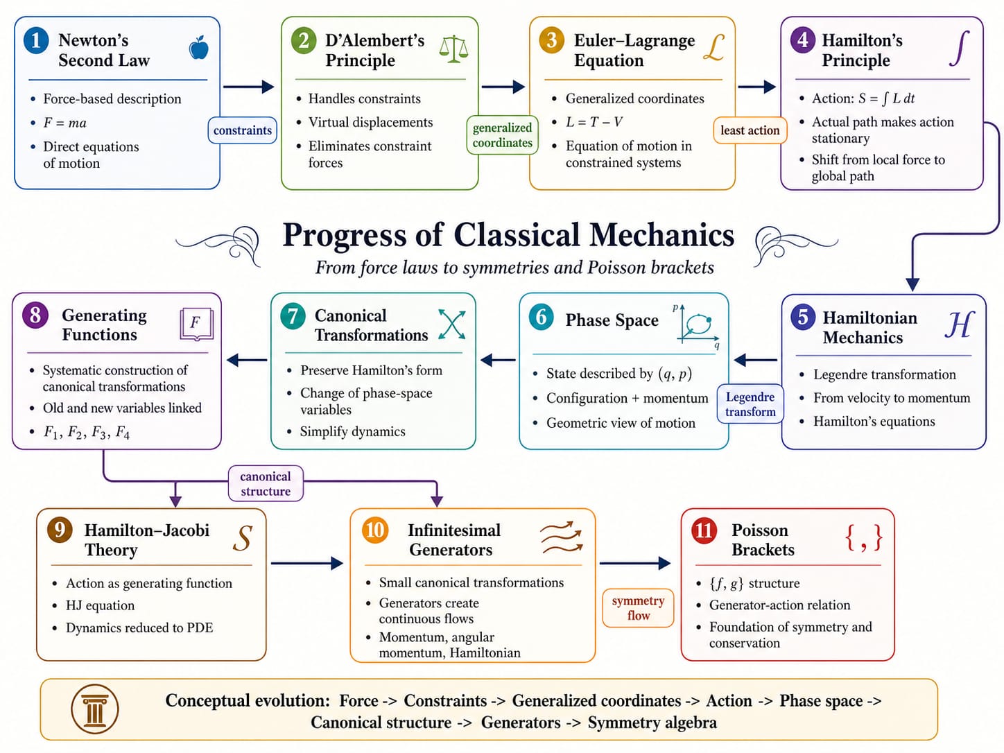
Thus the flow of ideas is:</p>

<ul>
  <li>canonical transformations preserve Hamiltonian structure,</li>
  <li>infinitesimal canonical transformations are generated by phase-space functions,</li>
  <li>Lie transformations are finite transformations built from infinitesimal ones,</li>
  <li>the Hamiltonian generates time translation,</li>
  <li>symmetry generators give conserved quantities,</li>
  <li>action-angle variables simplify bounded periodic motion.</li>
</ul>

<h2 id="infinitesimal-canonical-transformations-and-generators">Infinitesimal canonical transformations and generators</h2>

<p>Consider a type-$2$ generating function close to the identity transformation:</p>

\[F_2(q_i,P_i,t)=\sum_i q_iP_i+\varepsilon G(q_i,P_i,t)\]

<p>where $\varepsilon$ is a small parameter and $G$ is the infinitesimal generator. The transformation equations are</p>

\[p_i=\frac{\partial F_2}{\partial q_i},
\qquad
Q_i=\frac{\partial F_2}{\partial P_i}.\]

<p>Using the given $F_2$,</p>

\[p_i=P_i+\varepsilon\frac{\partial G}{\partial q_i}\]

<p>and</p>

\[Q_i=q_i+\varepsilon\frac{\partial G}{\partial P_i}.\]

<p>Since the transformation is infinitesimal, we may replace $P_i$ by $p_i$ in the first-order correction. Hence</p>

\[P_i=p_i-\varepsilon\frac{\partial G}{\partial q_i}\]

<p>and</p>

\[Q_i=q_i+\varepsilon\frac{\partial G}{\partial p_i}.\]

<p>Therefore the infinitesimal changes are</p>

\[\delta q_i=Q_i-q_i=\varepsilon\frac{\partial G}{\partial p_i},
\qquad
\delta p_i=P_i-p_i=-\varepsilon\frac{\partial G}{\partial q_i}.\]

<p>These are exactly the canonical transformation rules generated by $G$. They show that a single function $G(q,p,t)$ determines how every coordinate and momentum changes.</p>

<p>For any phase-space function $f(q_i,p_i,t)$, the infinitesimal change is</p>

\[\delta f
=
\sum_i\left(
\frac{\partial f}{\partial q_i}\delta q_i
+
\frac{\partial f}{\partial p_i}\delta p_i
\right).\]

<p>Substituting $\delta q_i$ and $\delta p_i$,</p>

\[\delta f
=
\varepsilon
\sum_i
\left(
\frac{\partial f}{\partial q_i}\frac{\partial G}{\partial p_i}
-
\frac{\partial f}{\partial p_i}\frac{\partial G}{\partial q_i}
\right).\]

<p>The expression in brackets is the Poisson bracket ${f,G}$. Therefore</p>

\[\boxed{
\delta f=\varepsilon\{f,G\}
}\]

<p>This is the central formula of infinitesimal canonical transformations. It says that the generator $G$ gives the direction of motion of every phase-space function through the Poisson bracket.</p>

<div style="border:2px solid #444; padding:16px; border-radius:8px; background:#fafafa;">

<p><b>Example: coordinate translation</b></p>

<p>Let the generator be</p>

$$
G=p.
$$

<p>Then for one degree of freedom,</p>

$$
\delta q=\varepsilon\{q,p\}=\varepsilon,
\qquad
\delta p=\varepsilon\{p,p\}=0.
$$

<p>Hence</p>

$$
q'=q+\varepsilon,
\qquad
p'=p.
$$

<p>Thus the generator $p$ produces a translation in the coordinate $q$. This is why momentum is called the generator of spatial translation.</p>

</div>

<h2 id="lie-transformations-from-infinitesimal-generators">Lie transformations from infinitesimal generators</h2>

<p>An infinitesimal transformation gives only a very small change. But if the same infinitesimal transformation is applied repeatedly, it builds a finite transformation. This finite transformation is called a Lie transformation.</p>

<p>Define the Lie operator $L_G$ by</p>

\[L_G f=\{f,G\}.\]

<p>Then one infinitesimal transformation gives</p>

\[f\longrightarrow f+\varepsilon L_G f.\]

<p>Repeated application gives the exponential form</p>

\[f'=\exp(\varepsilon L_G)f.\]

<p>Expanding the exponential,</p>

\[f'
=
f+\varepsilon L_Gf+\frac{\varepsilon^2}{2!}L_G^2f+\frac{\varepsilon^3}{3!}L_G^3f+\cdots.\]

<p>Since $L_Gf=\{f,G\}$, this becomes</p>

\[f'
=
f+\varepsilon\{f,G\}
+\frac{\varepsilon^2}{2!}\{\{f,G\},G\}
+\frac{\varepsilon^3}{3!}\{\{\{f,G\},G\},G\}
+\cdots.\]

<p>Thus a Lie transformation is not a separate kind of transformation. It is the finite transformation obtained by integrating or repeating the infinitesimal canonical transformation generated by $G$.</p>

<p>This is especially useful in perturbation theory. Instead of trying to find one large exact transformation, one chooses a generator that removes or simplifies undesirable terms order by order. In this way, Lie transformations provide a systematic method for simplifying Hamiltonians.</p>

<div style="border:2px solid #444; padding:16px; border-radius:8px; background:#fafafa;">

<p><b>Example: finite coordinate translation</b></p>

<p>Again take</p>

$$
G=p.
$$

<p>For the coordinate $q$,</p>

$$
L_Gq=\{q,p\}=1.
$$

<p>Applying the operator again,</p>

$$
L_G^2q=L_G(1)=\{1,p\}=0.
$$

<p>Therefore all higher terms vanish, and</p>

$$
q'=\exp(\varepsilon L_G)q=q+\varepsilon.
$$

<p>For the momentum $p$,</p>

$$
L_Gp=\{p,p\}=0.
$$

<p>Therefore</p>

$$
p'=\exp(\varepsilon L_G)p=p.
$$

<p>Hence the finite Lie transformation generated by $G=p$ is</p>

$$
\boxed{
q'=q+\varepsilon,\qquad p'=p.
}
$$

<p>This confirms that the generator $p$ produces a finite translation of the coordinate.</p>

</div>

<h2 id="the-hamiltonian-as-the-generator-of-time-translation">The Hamiltonian as the generator of time translation</h2>

<p>The Hamiltonian has a special role because it generates time evolution. Take the generator to be</p>

\[G=H\]

<p>and choose the small parameter to be</p>

\[\varepsilon=dt.\]

<p>Then</p>

\[\delta q_i=dt\{q_i,H\}\]

<p>and</p>

\[\delta p_i=dt\{p_i,H\}.\]

<p>Using the definition of the Poisson bracket,</p>

\[\{q_i,H\}=\frac{\partial H}{\partial p_i}\]

<p>and</p>

\[\{p_i,H\}=-\frac{\partial H}{\partial q_i}.\]

<p>Therefore</p>

\[\delta q_i=dt\frac{\partial H}{\partial p_i},
\qquad
\delta p_i=-dt\frac{\partial H}{\partial q_i}.\]

<p>Dividing by $dt$,</p>

\[\boxed{
\dot q_i=\frac{\partial H}{\partial p_i},
\qquad
\dot p_i=-\frac{\partial H}{\partial q_i}.
}\]

<p>These are Hamilton’s equations. Therefore the Hamiltonian is the generator of time translation in phase space.</p>

<p>This result gives a powerful interpretation of dynamics: time evolution itself is a canonical transformation generated by the Hamiltonian.</p>

<p>For any function $f(q,p,t)$,</p>

\[\frac{df}{dt}
=
\{f,H\}+\frac{\partial f}{\partial t}.\]

<p>If $f$ has no explicit time dependence, then</p>

\[\frac{df}{dt}=\{f,H\}.\]

<p>So the Hamiltonian flow tells how every observable changes with time.</p>

<h2 id="symmetry-and-conservation-laws-in-hamiltonian-form">Symmetry and conservation laws in Hamiltonian form</h2>

<p>A symmetry is a transformation that leaves the physical structure of the system unchanged. In Hamiltonian mechanics, a continuous symmetry is represented by a generator $G(q,p,t)$. The infinitesimal change of the Hamiltonian under this transformation is</p>

\[\delta H=\varepsilon\{H,G\}.\]

<p>If the Hamiltonian is invariant under the transformation, then</p>

\[\delta H=0.\]

<p>Therefore</p>

\[\{H,G\}=0.\]

<p>Since the Poisson bracket is antisymmetric,</p>

\[\{H,G\}=-\{G,H\}.\]

<p>So the invariance condition may also be written as</p>

\[\{G,H\}=0.\]

<p>Now the total time derivative of $G$ is</p>

\[\frac{dG}{dt}
=
\{G,H\}+\frac{\partial G}{\partial t}.\]

<p>If $G$ has no explicit time dependence and the Hamiltonian is invariant under the transformation generated by $G$, then</p>

\[\frac{dG}{dt}=0.\]

<p>Therefore</p>

\[\boxed{
G=\text{constant}.
}\]

<p>This is the Hamiltonian form of Noether’s theorem:</p>

\[\boxed{
\text{continuous symmetry}
\quad\Longrightarrow\quad
\text{conserved generator}.
}\]

<p>The important point is that a conserved quantity is not merely a number that accidentally remains constant. It is the generator of a continuous canonical symmetry.</p>

<p>The logic is:</p>

<ul>
  <li>$G$ generates an infinitesimal canonical transformation,</li>
  <li>the change of any phase-space function is $\delta f=\varepsilon{f,G}$,</li>
  <li>if the Hamiltonian is invariant under this transformation, then ${G,H}=0$,</li>
  <li>if $G$ has no explicit time dependence, then $\frac{dG}{dt}=0$,</li>
  <li>therefore $G$ is conserved.</li>
</ul>

<div style="border:2px solid #444; padding:16px; border-radius:8px; background:#fafafa;">

<p><b>Examples of symmetry generators</b></p>

<p><b>1. Spatial translation</b></p>

<p>If</p>

$$
G=p,
$$

<p>then</p>

$$
\delta q=\varepsilon,
\qquad
\delta p=0.
$$

<p>So $p$ generates spatial translation. If the Hamiltonian does not change under spatial translation, then</p>

$$
\{p,H\}=0
$$

<p>and therefore</p>

$$
p=\text{constant}.
$$

<p>Thus translational symmetry gives conservation of momentum.</p>

<hr />

<p><b>2. Rotation about the $z$-axis</b></p>

<p>If</p>

$$
G=L_z=xp_y-yp_x,
$$

<p>then $G$ generates rotation about the $z$-axis. If the Hamiltonian is invariant under this rotation, then</p>

$$
\{L_z,H\}=0
$$

<p>and therefore</p>

$$
L_z=\text{constant}.
$$

<p>Thus rotational symmetry gives conservation of angular momentum.</p>

<hr />

<p><b>3. Time translation</b></p>

<p>If the Hamiltonian has no explicit time dependence, then</p>

$$
\frac{\partial H}{\partial t}=0.
$$

<p>Using</p>

$$
\frac{dH}{dt}
=
\{H,H\}+\frac{\partial H}{\partial t},
$$

<p>and since</p>

$$
\{H,H\}=0,
$$

<p>we get</p>

$$
\frac{dH}{dt}=0.
$$

<p>Thus invariance under time translation gives conservation of energy.</p>

</div>

<h2 id="action-angle-variables">Action-angle variables</h2>

<p>Action-angle variables are special canonical variables designed for bounded periodic motion. They are useful because they convert complicated periodic motion into uniform motion.</p>

<p>The canonical transformation is</p>

\[(q_i,p_i)\longrightarrow(\theta_i,J_i),\]

<p>where $J_i$ are the action variables and $\theta_i$ are the corresponding angle variables.</p>

<p>The action variable tells which orbit the system is moving on. The angle variable tells where the system is on that orbit.</p>

<p>For one degree of freedom, periodic motion means</p>

\[q(t+T)=q(t),
\qquad
p(t+T)=p(t).\]

<p>Therefore the phase-space trajectory is a closed curve in the $(q,p)$ plane. Since the orbit is closed, we define the action variable by the closed integral</p>

\[\boxed{
J=\frac{1}{2\pi}\oint p\,dq.
}\]

<p>The integral $\oint p\,dq$ measures the phase-space area enclosed by the closed orbit. Since it is taken over the whole loop, it does not depend on the instantaneous position of the particle. It depends only on the orbit itself.</p>

<p>The factor $1/2\pi$ is introduced because the conjugate coordinate is an angle variable, and an angle increases by $2\pi$ in one complete cycle.</p>

<p>Thus:</p>

<ul>
  <li>$J$ labels the closed orbit,</li>
  <li>$\theta$ labels the position on that orbit,</li>
  <li>$J$ behaves like a momentum variable,</li>
  <li>$\theta$ behaves like a coordinate variable.</li>
</ul>

<p>For action-angle variables, the new Hamiltonian is chosen to depend only on $J$:</p>

\[K=K(J).\]

<p>Then Hamilton’s equations become</p>

\[\dot J=-\frac{\partial K}{\partial \theta}=0\]

<p>and</p>

\[\dot\theta=\frac{\partial K}{\partial J}=\omega(J).\]

<p>Therefore</p>

\[\boxed{
J=\text{constant},
\qquad
\theta(t)=\omega(J)t+\theta_0.
}\]

<p>This is the main advantage of action-angle variables. The original motion may be complicated in $(q,p)$, but in $(\theta,J)$ it becomes uniform motion with constant angular speed.</p>

<h2 id="why-the-action-variable-is-introduced">Why the action variable is introduced</h2>

<p>The formula</p>

\[J=\frac{1}{2\pi}\oint p\,dq\]

<p>should not be introduced as an isolated formula. It is meaningful only for systems with bounded periodic motion.</p>

<p>Such systems have the following features:</p>

<ul>
  <li>the motion is bounded,</li>
  <li>the motion repeats after a period,</li>
  <li>the phase trajectory is closed,</li>
  <li>different energies correspond to different closed phase-space loops,</li>
  <li>we want one variable that labels the whole orbit.</li>
</ul>

<p>For one degree of freedom, the instantaneous state is represented by $(q,p)$. During periodic motion, the phase point moves around a closed curve. Instead of asking where the particle is at a particular instant, we may ask which closed curve it is moving on. The action variable answers this second question.</p>

<p>The closed integral</p>

\[\oint p\,dq\]

<p>is natural because it is taken around the complete orbit. It measures the whole loop, not one point on the loop. Therefore it remains the same throughout the motion.</p>

<p>So the conceptual shift is:</p>

\[(q,p)
\quad\text{describes instantaneous state,}\]

<p>whereas</p>

\[J
\quad\text{describes the whole periodic orbit.}\]

<p>The conjugate angle variable $\theta$ then describes the running phase along the orbit.</p>

<h2 id="simple-harmonic-oscillator">Simple harmonic oscillator</h2>

<p>Consider the one-dimensional harmonic oscillator with Hamiltonian</p>

\[H=\frac{p^2}{2m}+\frac{1}{2}m\omega^2q^2.\]

<p>For a fixed energy $E$,</p>

\[E=\frac{p^2}{2m}+\frac{1}{2}m\omega^2q^2.\]

<p>Solving for $p$,</p>

\[p=\pm\sqrt{2mE-m^2\omega^2q^2}.\]

<p>The phase-space orbit is an ellipse. Its maximum coordinate is</p>

\[q_{\max}=A=\sqrt{\frac{2E}{m\omega^2}},\]

<p>and its maximum momentum is</p>

\[p_{\max}=m\omega A.\]

<p>The area enclosed by the ellipse is</p>

\[\oint p\,dq
=
\pi q_{\max}p_{\max}.\]

<p>Therefore</p>

\[\oint p\,dq
=
\pi A(m\omega A)
=
\pi m\omega A^2.\]

<p>The action variable is</p>

\[J=\frac{1}{2\pi}\oint p\,dq.\]

<p>Thus</p>

\[J
=
\frac{1}{2\pi}\pi m\omega A^2
=
\frac{1}{2}m\omega A^2.\]

<p>But for the harmonic oscillator,</p>

\[E=\frac{1}{2}m\omega^2A^2.\]

<p>Therefore</p>

\[\boxed{
J=\frac{E}{\omega}.
}\]

<p>Hence</p>

\[E=\omega J.\]

<p>So the transformed Hamiltonian is</p>

\[K(J)=\omega J.\]

<p>Hamilton’s equations are</p>

\[\dot J=-\frac{\partial K}{\partial \theta}=0\]

<p>and</p>

\[\dot\theta=\frac{\partial K}{\partial J}=\omega.\]

<p>Therefore</p>

\[\boxed{
J=\text{constant},
\qquad
\theta=\omega t+\theta_0.
}\]

<p>The harmonic oscillator, which appears as back-and-forth motion in $q$, becomes uniform phase motion in $\theta$.</p>

<h2 id="general-one-dimensional-potential-well">General one-dimensional potential well</h2>

<p>Consider a particle moving in a smooth potential $V(q)$ with Hamiltonian</p>

\[H=\frac{p^2}{2m}+V(q).\]

<p>Suppose the particle is trapped between two turning points $q_{\min}$ and $q_{\max}$, where</p>

\[V(q_{\min})=E,
\qquad
V(q_{\max})=E.\]

<p>From the energy equation,</p>

\[E=\frac{p^2}{2m}+V(q),\]

<p>we get</p>

\[p=\pm\sqrt{2m(E-V(q))}.\]

<p>The action variable is</p>

\[J=\frac{1}{2\pi}\oint p\,dq.\]

<p>For back-and-forth motion between the two turning points, the upper and lower halves of the closed phase curve contribute equally. Hence</p>

\[\boxed{
J(E)=
\frac{1}{\pi}
\int_{q_{\min}}^{q_{\max}}
\sqrt{2m(E-V(q))}\,dq.
}\]

<p>This expression is important because it works even when the exact solution $q(t)$ is difficult to find. The action variable can still be obtained from the geometry of the phase-space orbit.</p>

<p>Now we show that the angle variable grows with the physical frequency. Since the transformed Hamiltonian depends only on $J$,</p>

\[K=K(J)=E(J).\]

<p>Therefore</p>

\[\dot J=-\frac{\partial K}{\partial \theta}=0\]

<p>and</p>

\[\dot\theta=\frac{\partial K}{\partial J}=\frac{dE}{dJ}.\]

<p>Using the chain rule,</p>

\[\frac{dE}{dJ}
=
\left(\frac{dJ}{dE}\right)^{-1}.\]

<p>Now differentiate</p>

\[J(E)=
\frac{1}{\pi}
\int_{q_{\min}}^{q_{\max}}
\sqrt{2m(E-V(q))}\,dq.\]

<p>The endpoint terms vanish because the integrand becomes zero at the turning points. Therefore</p>

\[\frac{dJ}{dE}
=
\frac{1}{\pi}
\int_{q_{\min}}^{q_{\max}}
\frac{m}{\sqrt{2m(E-V(q))}}\,dq.\]

<p>Since</p>

\[p=\sqrt{2m(E-V(q))}\]

<p>and</p>

\[\dot q=\frac{p}{m},\]

<p>we have</p>

\[\frac{m}{\sqrt{2m(E-V(q))}}
=
\frac{m}{p}
=
\frac{1}{\dot q}.\]

<p>Therefore</p>

\[\frac{dJ}{dE}
=
\frac{1}{\pi}
\int_{q_{\min}}^{q_{\max}}
\frac{dq}{\dot q}.\]

<p>But</p>

\[\int_{q_{\min}}^{q_{\max}}
\frac{dq}{\dot q}\]

<p>is the time taken to move from one turning point to the other. This is half the period:</p>

\[\int_{q_{\min}}^{q_{\max}}
\frac{dq}{\dot q}
=
\frac{T}{2}.\]

<p>Hence</p>

\[\frac{dJ}{dE}
=
\frac{1}{\pi}\frac{T}{2}
=
\frac{T}{2\pi}.\]

<p>Therefore</p>

\[\frac{dE}{dJ}
=
\frac{2\pi}{T}.\]

<p>Thus</p>

\[\boxed{
\dot\theta=\omega=\frac{2\pi}{T}.
}\]

<p>So for any one-dimensional bounded periodic system,</p>

\[\boxed{
\dot J=0,
\qquad
\dot\theta=\omega.
}\]

<p>This proves that action-angle variables convert general periodic motion into uniform angular motion.</p>

<h2 id="small-angle-pendulum">Small-angle pendulum</h2>

<p>For a pendulum of length $l$ and mass $m$, the exact Hamiltonian is</p>

\[H=\frac{p_\theta^2}{2ml^2}+mgl(1-\cos\theta).\]

<p>For small oscillations,</p>

\[\cos\theta\simeq 1-\frac{\theta^2}{2}.\]

<p>Therefore</p>

\[mgl(1-\cos\theta)\simeq \frac{1}{2}mgl\theta^2.\]

<p>The Hamiltonian becomes</p>

\[H=
\frac{p_\theta^2}{2ml^2}
+
\frac{1}{2}mgl\theta^2.\]

<p>This is mathematically equivalent to a harmonic oscillator with angular frequency</p>

\[\omega=\sqrt{\frac{g}{l}}.\]

<p>Therefore the action variable is</p>

\[J=\frac{1}{2\pi}\oint p_\theta\,d\theta.\]

<p>Using the harmonic oscillator result,</p>

\[\boxed{
J=\frac{E}{\omega}
=
E\sqrt{\frac{l}{g}}.
}\]

<p>The transformed Hamiltonian is</p>

\[K(J)=\omega J,
\qquad
\omega=\sqrt{\frac{g}{l}}.\]

<p>Therefore</p>

\[\dot J=-\frac{\partial K}{\partial \theta}=0\]

<p>and</p>

\[\dot\theta=\frac{\partial K}{\partial J}=\omega.\]

<p>Hence</p>

\[\boxed{
\dot J=0,
\qquad
\dot\theta=\sqrt{\frac{g}{l}}.
}\]

<p>Thus the small-angle pendulum becomes uniform phase motion in action-angle variables.</p>

<h2 id="practice-questions">Practice questions</h2>

<p>Q1. Starting from</p>

\[F_2(q_i,P_i,t)=\sum_i q_iP_i+\varepsilon G(q_i,P_i,t),\]

<p>derive the infinitesimal canonical transformation formulas.</p>

<p>Q2. Prove that for any phase-space function $f(q_i,p_i,t)$,</p>

\[\delta f=\varepsilon\{f,G\}.\]

<p>Q3. Show explicitly that choosing $G=H$ and $\varepsilon=dt$ reproduces Hamilton’s equations.</p>

<p>Q4. Explain why the Hamiltonian is called the generator of time translation.</p>

<p>Q5. If $G$ has no explicit time dependence and satisfies</p>

\[\{G,H\}=0,\]

<p>show that $G$ is conserved.</p>

<p>Q6. Show that momentum generates spatial translation.</p>

<p>Q7. Show that $L_z=xp_y-yp_x$ generates rotation about the $z$-axis.</p>

<p>Q8. Explain why translational symmetry gives conservation of momentum.</p>

<p>Q9. Explain why rotational symmetry gives conservation of angular momentum.</p>

<p>Q10. For the harmonic oscillator, show that</p>

\[J=\frac{E}{\omega}.\]

<p>Q11. For a general one-dimensional potential well, prove that</p>

\[\frac{dJ}{dE}=\frac{T}{2\pi}.\]

<p>Q12. Hence prove that</p>

\[\dot\theta=\frac{dE}{dJ}=\frac{2\pi}{T}.\]

<p>Q13. For the small-angle pendulum, show that</p>

\[J=E\sqrt{\frac{l}{g}}.\]

<p>Q14. Explain why action-angle variables convert bounded periodic motion into uniform phase motion.</p>

<p>Q15. Explain the statement: conserved quantities are generators of continuous canonical symmetries.</p>]]></content><author><name>Rajesh Kumar</name></author><category term="notes" /><category term="msc" /><category term="msc-i" /><category term="lecture" /><category term="msc" /><category term="semester-i" /><category term="classical-mechanics" /><category term="symmetry" /><category term="noether" /><category term="action-angle" /><summary type="html"><![CDATA[In Hamiltonian mechanics, canonical transformations are important because they preserve the form of Hamilton’s equations. If the old canonical variables $(q_i,p_i)$ are replaced by new variables $(Q_i,P_i)$, the transformation is canonical only when the new variables also satisfy Hamilton’s equations in the same structural form. This allows us to change variables without changing the basic geometry of mechanics.]]></summary></entry><entry><title type="html">Canonical Maps</title><link href="https://rajeshphy.github.io/msc/sem-i/canonical-maps/" rel="alternate" type="text/html" title="Canonical Maps" /><published>2026-05-04T03:40:00+00:00</published><updated>2026-05-04T03:40:00+00:00</updated><id>https://rajeshphy.github.io/msc/sem-i/canonical-maps</id><content type="html" xml:base="https://rajeshphy.github.io/msc/sem-i/canonical-maps/"><![CDATA[<p>Hamilton–Jacobi theory naturally extends to canonical transformations because the action function $S$ itself behaves like a generating function. This extension clarifies why Hamiltonian mechanics can be simplified by changing phase-space variables and how continuous symmetry transformations arise from infinitesimal generators.</p>

<h2 id="canonical-transformations">Canonical transformations</h2>

<p>In Hamiltonian mechanics, the state of a system is described by canonical coordinates and momenta $(q_i,p_i)$. A transformation to new variables $(Q_i,P_i)$ is called a canonical transformation <strong>if the new variables also satisfy Hamilton’s equations in canonical form.</strong> The importance of such transformations is that they preserve the structure of mechanics while possibly making the problem much simpler.</p>

<p>The differential form of Hamilton’s principal function is</p>

\[dS=\sum_i p_i\,dq_i-H\,dt\]

<p>Suppose we transform to new variables $(Q_i,P_i)$ with a new Hamiltonian $K$. Then the corresponding canonical differential form is</p>

\[dS'=\sum_i P_i\,dQ_i-K\,dt\]

<p>A transformation is canonical if the difference between the old and new one-forms is an exact differential. Thus one requires</p>

\[\sum_i p_i\,dq_i-H\,dt-\left(\sum_i P_i\,dQ_i-K\,dt\right)=dF\]

<p>where $F$ is some function. <strong>This is the basic condition for a canonical transformation.</strong> It means that the equations of motion preserve their Hamiltonian form under the transformation.</p>

<p>Thus canonical transformations preserve the symplectic structure of phase space. They do not merely change coordinates; they preserve the dynamical framework itself.</p>

<div style="background:linear-gradient(135deg,#f8fbff 0%,#eef4ff 100%); border:1px solid #d6e4ff; border-radius:18px; padding:22px; box-shadow:0 10px 30px rgba(30,60,120,0.08);">


Starting with the canonical condition

$$
\sum_i p_i\,dq_i-\sum_i P_i\,dQ_i+(K-H)\,dt=dF
$$

We decide which variables $F$ depends on, we expand $dF$ in terms of those variables and then compare coefficients of the independent differentials.

For example, if

$$
F_1=F_1(q_i,Q_i,t)
$$

then its exact differential is

$$
dF_1=\sum_i \frac{\partial F_1}{\partial q_i}\,dq_i+\sum_i \frac{\partial F_1}{\partial Q_i}\,dQ_i+\frac{\partial F_1}{\partial t}\,dt
$$

But from the canonical condition,

$$
dF_1=\sum_i p_i\,dq_i-\sum_i P_i\,dQ_i+(K-H)\,dt
$$

Now compare coefficients of the same independent differentials:
<ul>
  <li>coefficient of $dq_i$:</li>
</ul>

$$
\frac{\partial F_1}{\partial q_i}=p_i
$$

<ul>
  <li>coefficient of $dQ_i$:</li>
</ul>

$$
\frac{\partial F_1}{\partial Q_i}=-P_i
$$

<ul>
  <li>coefficient of $dt$:</li>
</ul>

$$
\frac{\partial F_1}{\partial t}=K-H
$$
Hence

$$
p_i=\frac{\partial F_1}{\partial q_i},\qquad
P_i=-\frac{\partial F_1}{\partial Q_i},\qquad
K=H+\frac{\partial F_1}{\partial t}
$$

That is what is meant by “expand $dF$ and compare coefficients.”
<br />
<strong>Now suppose we do not want the generating function in terms of $Q_i$.</strong> We want a new generating function in terms of $P_i$ instead. Since $P_i$ is related to $Q_i$ by

$$

P_i=-\frac{\partial F_1}{\partial Q_i}

$$

the natural way to replace the variable $Q_i$ by its conjugate quantity $P_i$ is by a <strong>Legendre transform</strong>.

So define

$$

F_2(q_i,P_i,t)=F_1(q_i,Q_i,t)+\sum_i Q_iP_i

$$

This is exactly the Legendre transformation of $F_1$ with respect to $Q_i$ because:
<ul>
    <li> old independent variable: $Q_i$ </li>

    <li> conjugate derivative variable: $-P_i=\dfrac{\partial F_1}{\partial Q_i}$ </li>
</ul>

The plus sign appears because

$$

P_i=-\frac{\partial F_1}{\partial Q_i}

$$

If the sign had been positive, the Legendre term would have appeared with a minus sign instead.


Now differentiate:

$$
dF_2=dF_1+\sum_i Q_i\,dP_i+\sum_i P_i\,dQ_i
$$

Using the canonical condition for $F_1$,

$$
dF_1=\sum_i p_i\,dq_i-\sum_i P_i\,dQ_i+(K-H)\,dt
$$

we get

$$
dF_2=\sum_i p_i\,dq_i+\sum_i Q_i\,dP_i+(K-H)\,dt
$$

Since $F_2=F_2(q_i,P_i,t)$, its exact differential is also

$$
dF_2=\sum_i \frac{\partial F_2}{\partial q_i}\,dq_i+\sum_i \frac{\partial F_2}{\partial P_i}\,dP_i+\frac{\partial F_2}{\partial t}\,dt
$$

Now compare coefficients of the independent differentials $dq_i$, $dP_i$, and $dt$. This gives

$$
p_i=\frac{\partial F_2}{\partial q_i},\qquad
Q_i=\frac{\partial F_2}{\partial P_i},\qquad
K=H+\frac{\partial F_2}{\partial t}
$$

So here “expansion” means writing the total differential of $F_2$ in its chosen variables, but the crucial missing step is that the canonical one-form must first be rewritten in terms of $dq_i$, $dP_i$, and $dt$.


</div>

<h2 id="generating-functions">Generating functions</h2>

<p>The function $F$ appearing above is called a generating function. Depending on which old and new variables are chosen as independent arguments, there are four standard types of generating functions.</p>
<div style="background:linear-gradient(135deg,#f8fbff 0%,#eef4ff 100%); border:1px solid #d6e4ff; border-radius:18px; padding:22px; box-shadow:0 10px 30px rgba(30,60,120,0.08);">

  <div style="text-align:center; margin-bottom:18px;">
    <span style="display:inline-block; background:#2b6cb0; color:white; padding:8px 18px; border-radius:999px; font-size:0.95rem; font-weight:700; letter-spacing:0.5px;">
      Generating Functions: Four Standard Forms
    </span>
  </div>

  <div style="display:grid; gap:16px;">

    <div style="background:white; border-left:6px solid #2b6cb0; border-radius:14px; padding:16px 18px; box-shadow:0 4px 14px rgba(0,0,0,0.05);">
      <p style="margin:0 0 10px 0; font-size:1.05rem; font-weight:700; color:#1a365d;">
        If $F_1 = F_1(q,Q,t)$, then
      </p>
      <div style="background:#f7faff; border-radius:10px; padding:12px 14px;">
        $$
        p_i=\frac{\partial F_1}{\partial q_i}, \qquad
        P_i=-\frac{\partial F_1}{\partial Q_i}, \qquad
        K=H+\frac{\partial F_1}{\partial t}
        $$
      </div>
    </div>

    <div style="background:white; border-left:6px solid #38a169; border-radius:14px; padding:16px 18px; box-shadow:0 4px 14px rgba(0,0,0,0.05);">
      <p style="margin:0 0 10px 0; font-size:1.05rem; font-weight:700; color:#22543d;">
        If $F_2 = F_2(q,P,t)$, then
      </p>
      <div style="background:#f7fff9; border-radius:10px; padding:12px 14px;">
        $$
        p_i=\frac{\partial F_2}{\partial q_i}, \qquad
        Q_i=\frac{\partial F_2}{\partial P_i}, \qquad
        K=H+\frac{\partial F_2}{\partial t}
        $$
      </div>
    </div>

    <div style="background:white; border-left:6px solid #d69e2e; border-radius:14px; padding:16px 18px; box-shadow:0 4px 14px rgba(0,0,0,0.05);">
      <p style="margin:0 0 10px 0; font-size:1.05rem; font-weight:700; color:#744210;">
        If $F_3 = F_3(p,Q,t)$, then
      </p>
      <div style="background:#fffdf7; border-radius:10px; padding:12px 14px;">
        $$
        q_i=-\frac{\partial F_3}{\partial p_i}, \qquad
        P_i=-\frac{\partial F_3}{\partial Q_i}, \qquad
        K=H+\frac{\partial F_3}{\partial t}
        $$
      </div>
    </div>

    <div style="background:white; border-left:6px solid #805ad5; border-radius:14px; padding:16px 18px; box-shadow:0 4px 14px rgba(0,0,0,0.05);">
      <p style="margin:0 0 10px 0; font-size:1.05rem; font-weight:700; color:#44337a;">
        If $F_4 = F_4(p,P,t)$, then
      </p>
      <div style="background:#faf7ff; border-radius:10px; padding:12px 14px;">
        $$
        q_i=-\frac{\partial F_4}{\partial p_i}, \qquad
        Q_i=\frac{\partial F_4}{\partial P_i}, \qquad
        K=H+\frac{\partial F_4}{\partial t}
        $$
      </div>
    </div>

  </div>
</div>
<p>Among these, the type-$2$ generating function is especially important in Hamilton–Jacobi theory. If one writes</p>

\[F_2(q,P,t)=S(q,P,t)\]

<p>then</p>

\[p_i=\frac{\partial S}{\partial q_i}, \qquad
Q_i=\frac{\partial S}{\partial P_i}\]

<p>If the new Hamiltonian is chosen to vanish,</p>

\[K=K(Q,P)=0\]

<p>then the condition</p>

\[K=H+\frac{\partial S}{\partial t}=0\]

<p>becomes</p>

\[\frac{\partial S}{\partial t}+H\left(q_i,\frac{\partial S}{\partial q_i},t\right)=0\]

<p>which is precisely the Hamilton–Jacobi equation. <strong>Thus Hamilton–Jacobi theory is the special case of a canonical transformation generated by $S$ that transforms the dynamics into a trivial one with constant new variables.</strong></p>

<p>This also explains the origin of the constants in Hamilton–Jacobi theory. If $P_i=\alpha_i$, then</p>

\[Q_i=\frac{\partial S}{\partial \alpha_i}=\beta_i\]

<p>and because $K=0$, Hamilton’s equations in the new variables give</p>

\[\dot p_i=0, \qquad \dot Q_i=0\]

<p>Hence both $\alpha_i$ and $\beta_i$ are constants.</p>

<h2 id="infinitesimal-canonical-transformations">Infinitesimal Canonical Transformations</h2>

<p>Take an infinitesimal canonical transformation as one which is very close to the identity transformation:</p>

\[Q_i=q_i+\delta q_i,\qquad P_i=p_i+\delta p_i\]

<p>where $\delta q_i$ and $\delta p_i$ are very small quantities of first order in a small parameter $\varepsilon$.</p>

<p>Now begin with a <strong>type-2 generating function</strong> and choose it in the form</p>

\[F_2(q,P,t)=\sum_i q_iP_i+\varepsilon G(q,P,t)\]

<p>Here:</p>

<ul>
  <li>$\sum_i q_iP_i$ gives the identity transformation</li>
  <li>$\varepsilon G$ gives a small deviation from identity</li>
  <li>$G$ is called the <strong>infinitesimal generator</strong></li>
</ul>

<p><strong>Why $\sum_i q_iP_i$ gives identity</strong></p>

<p>For a type-2 generating function, the transformation equations are</p>

\[p_i=\frac{\partial F_2}{\partial q_i},\qquad
Q_i=\frac{\partial F_2}{\partial P_i}\]

<p>If</p>

\[F_2=\sum_i q_iP_i\]

<p>then</p>

\[p_i=P_i,\qquad Q_i=q_i\]

<p>So the old and new variables are the same. Hence this is the identity transformation.</p>

<p><strong>Add a small correction</strong></p>

<p>Now take</p>

\[F_2(q,P,t)=\sum_i q_iP_i+\varepsilon G(q,P,t)\]

<p>Then</p>

\[p_i=\frac{\partial F_2}{\partial q_i}
= P_i+\varepsilon \frac{\partial G}{\partial q_i}\]

<p>and</p>

\[Q_i=\frac{\partial F_2}{\partial P_i}
= q_i+\varepsilon \frac{\partial G}{\partial P_i}\]

<p>Since the transformation is infinitesimal, the difference between $P_i$ and $p_i$ is already of order $\varepsilon$. Therefore, inside first-order terms, we may replace $P_i$ by $p_i$. Thus</p>

\[Q_i=q_i+\varepsilon \frac{\partial G}{\partial p_i}\]

<p>Hence</p>

\[\delta q_i=Q_i-q_i=\varepsilon \frac{\partial G}{\partial p_i}\]

<p>Now from</p>

\[p_i=P_i+\varepsilon \frac{\partial G}{\partial q_i}\]

<p>we get</p>

\[P_i=p_i-\varepsilon \frac{\partial G}{\partial q_i}\]

<p>Therefore</p>

\[\delta p_i=P_i-p_i=-\varepsilon \frac{\partial G}{\partial q_i}\]

<p>So the infinitesimal canonical transformation is</p>

\[\boxed{\delta q_i=\varepsilon \frac{\partial G}{\partial p_i},\qquad
\delta p_i=-\varepsilon \frac{\partial G}{\partial q_i}}\]

<h2 id="why-this-looks-like-hamiltons-equations">Why this looks like Hamilton’s equations</h2>

<p>Hamilton’s equations are</p>

\[\dot q_i=\frac{\partial H}{\partial p_i},\qquad
\dot p_i=-\frac{\partial H}{\partial q_i}\]

<p>Now compare with</p>

\[\delta q_i=\varepsilon \frac{\partial G}{\partial p_i},\qquad
\delta p_i=-\varepsilon \frac{\partial G}{\partial q_i}\]

<p>Dividing by $\varepsilon$,</p>

\[\frac{\delta q_i}{\varepsilon}=\frac{\partial G}{\partial p_i},\qquad
\frac{\delta p_i}{\varepsilon}=-\frac{\partial G}{\partial q_i}\]

<p>This has exactly the same structure as Hamilton’s equations, except that:</p>

<ul>
  <li>$H$ is replaced by $G$</li>
  <li>time $t$ is replaced by the transformation parameter $\varepsilon$</li>
</ul>

<p>So $G$ generates motion in phase space with respect to $\varepsilon$, just as $H$ generates motion with respect to time.</p>

<h2 id="main-idea">Main idea</h2>

<ul>
  <li>$H$ generates <strong>time evolution</strong></li>
  <li>$G$ generates a <strong>canonical transformation</strong></li>
  <li>infinitesimal means the transformation is only a very small step away from identity</li>
  <li>a finite canonical transformation can be built by repeating many such infinitesimal steps</li>
</ul>

<p>These relations have exactly the same form as Hamilton’s equations, except that the evolution parameter is now $\varepsilon$ instead of time.</p>

<p>Using Poisson brackets, these can be written compactly as</p>

\[\delta q_i=\varepsilon \{q_i,G\}, \qquad
\delta p_i=\varepsilon \{p_i,G\}\]

<p>and for any dynamical quantity $f(q,p,t)$,</p>

\[\delta f=\varepsilon \{f,G\}\]

<p>Thus the infinitesimal generator produces canonical transformations through Poisson brackets. This is the phase-space analogue of the way a generator produces a continuous symmetry in other branches of physics.</p>

<h2 id="meaning-of-the-generator">Meaning of the generator</h2>

<p>The generator $G$ determines the direction in which the phase-space point moves under the infinitesimal transformation. Different choices of $G$ produce different transformations.</p>

<p>If</p>

\[G=p\]

<p>for one degree of freedom, then</p>

\[\delta q=\varepsilon, \qquad \delta p=0\]

<p>which is a translation in coordinate.</p>

<p>If</p>

\[G=-q\]

<p>then</p>

\[\delta q=0, \qquad \delta p=\varepsilon\]

<p>which is a translation in momentum.</p>

<p>If the Hamiltonian itself acts as the generator, then</p>

\[\delta q_i=\varepsilon \frac{\partial H}{\partial p_i}, \qquad
\delta p_i=-\varepsilon \frac{\partial H}{\partial q_i}\]

<p>which is exactly the time development of the system for an interval $\varepsilon$. Therefore the Hamiltonian is the generator of time evolution.</p>

<h2 id="relation-with-poisson-brackets-and-conservation-laws">Relation with Poisson brackets and conservation laws</h2>

<p>For any quantity $f(q,p,t)$, the total time evolution is</p>

\[\frac{df}{dt}=\{f,H\}+\frac{\partial f}{\partial t}\]

<p>If a quantity $G$ has no explicit time dependence and satisfies</p>

\[\{G,H\}=0\]

<p>then</p>

\[\frac{dG}{dt}=0\]

<p>so $G$ is conserved. Hence conserved quantities are deeply connected with generators. A symmetry generator that leaves the Hamiltonian unchanged gives a constant of motion.</p>

<p>This idea links canonical transformations with conservation laws and prepares the way for more advanced ideas such as action-angle variables, Lie transformations, and Noether-type symmetry analysis in Hamiltonian form.</p>

<h2 id="main-points">Main points</h2>

<ul>
  <li>A canonical transformation preserves Hamilton’s equations in canonical form.</li>
  <li>The condition for canonicity is that the difference of the old and new phase-space one-forms is an exact differential.</li>
  <li>That exact differential defines a generating function.</li>
  <li>There are four standard types of generating functions.</li>
  <li>Hamilton–Jacobi theory is a special canonical transformation generated by $S$ with new Hamiltonian $K=0$.</li>
  <li>Infinitesimal canonical transformations are generated by a function $G$.</li>
  <li>The change of any quantity under an infinitesimal canonical transformation is given by its Poisson bracket with $G$.</li>
  <li>The Hamiltonian itself is the generator of time evolution.</li>
</ul>

<h2 id="practice-questions">Practice questions</h2>

<ol>
  <li>Show that a transformation is canonical if the difference between the old and new phase-space one-forms is an exact differential.</li>
  <li>Derive the relations for the type-$2$ generating function $F_2(q,P,t)$.</li>
  <li>Explain how Hamilton’s principal function $S$ acts as a generating function in Hamilton–Jacobi theory.</li>
  <li>Prove that an infinitesimal canonical transformation generated by $G$ preserves Poisson bracket structure.</li>
  <li>Show that the Hamiltonian generates time translations in phase space.</li>
</ol>]]></content><author><name>Rajesh Kumar</name></author><category term="notes" /><category term="msc" /><category term="msc-i" /><category term="lecture" /><category term="msc" /><category term="semester-i" /><category term="classical-mechanics" /><category term="canonical-transformations" /><category term="generating-functions" /><summary type="html"><![CDATA[Hamilton–Jacobi theory naturally extends to canonical transformations because the action function $S$ itself behaves like a generating function. This extension clarifies why Hamiltonian mechanics can be simplified by changing phase-space variables and how continuous symmetry transformations arise from infinitesimal generators.]]></summary></entry></feed>