09 Jun 2026
Information Dynamics in Quantum Harmonic Systems VI: Quantum Control and Transport Fidelity
This post continues the complexity discussion, but now the model changes. The earlier posts studied two coupled oscillators, where synchronization, mutual information, and circuit depth were compared. Section 4 of the paper asks a more operational question:
If we physically transport a quantum state, how do fidelity, nonadiabatic excitation, and complexity compete?
The setting is deliberately simple: a single ion in a harmonic trap whose center is moved in time. Because the model is exactly solvable, it becomes a clean test case for the fidelity-complexity trade-off.
1. New Terms in This Section
Before entering the equations, let us fix the vocabulary. Section 4 introduces a new model and therefore a few new terms.
| Term | First meaning |
|---|---|
| quantum control | changing an external parameter in time to guide a quantum state |
| transport | moving a trapped quantum particle from one position to another |
| trap minimum | the point where the harmonic potential is smallest |
| protocol | the chosen time-profile of the control parameter |
| fidelity | overlap between the actual final state and the desired state |
| coherent state | a displaced ground state of a harmonic oscillator |
| displacement operator | the operator that shifts the oscillator in phase space |
| nonadiabaticity | amount of unwanted excitation caused by too-fast control |
| complexity | operational cost of preparing or reaching a state |
| TFD complexity | a complexity measure sensitive to displacement and temperature |
The earlier coupled-oscillator sections asked how correlations are generated. This section asks how a single state is moved while keeping it clean.
So the physical problem changes from one question to another:
| Earlier coupled-oscillator question | New one-body transport question |
|---|---|
| How correlated are two oscillators? | How accurately and cheaply can one oscillator be transported? |
2. Physical Picture
Imagine a harmonic trap whose minimum is not fixed at the origin. Instead, the minimum follows a prescribed trajectory $d(t)$. The ion feels a potential centered at $x=d(t)$.
The Hamiltonian is
\[\hat H(t) = \frac{\hat p^2}{2m} + \frac{1}{2}m\omega^2[\hat x-d(t)]^2.\]Here:
| Symbol | Meaning |
|---|---|
| $m$ | mass of the ion |
| $\omega$ | trap frequency |
| $\hat x,\hat p$ | position and momentum operators |
| $d(t)$ | externally controlled trap trajectory |
The control problem is this: move the trap from one place to another while keeping the ion as close as possible to the desired quantum state.
If the trap is moved too suddenly, the ion is excited. If it is moved smoothly, the ion can follow the trap more adiabatically.
This is called a one-body model because only one quantum particle is being transported. There is no second oscillator, no mutual information, and no two-body entanglement. The complexity here is not the cost of creating correlations between two modes. It is the cost of moving one mode without producing unwanted excitation.
3. Expanding the Hamiltonian
To see where the control enters, expand the potential:
\[[\hat x-d(t)]^2 = \hat x^2-2d(t)\hat x+d^2(t).\]Therefore
\[\hat H(t) = \frac{\hat p^2}{2m} + \frac{1}{2}m\omega^2\hat x^2 - m\omega^2d(t)\hat x + \frac{1}{2}m\omega^2d^2(t).\]The last term depends only on time. It contributes a global phase to the wavefunction and does not change the probability distribution. The physically important term is
\[-m\omega^2d(t)\hat x.\]This is a time-dependent force term. So a moving trap is equivalent to a harmonic oscillator driven by a force proportional to $d(t)$.
Term by term, the Hamiltonian says:
| Term | Physical role |
|---|---|
| $\hat p^2/(2m)$ | kinetic energy |
| $m\omega^2\hat x^2/2$ | ordinary harmonic trapping |
| $-m\omega^2d(t)\hat x$ | external time-dependent drive |
| $m\omega^2d^2(t)/2$ | time-dependent phase contribution |
Only the third term changes the oscillator’s motion. That is the first-principle origin of excitation in this model.
4. From Position Control to Ladder Operators
To connect the Hamiltonian with coherent states, write the position and momentum operators in terms of the creation and annihilation operators:
\[\hat x = \sqrt{\frac{\hbar}{2m\omega}} (\hat a+\hat a^\dagger),\]and
\[\hat p = -i\sqrt{\frac{m\hbar\omega}{2}} (\hat a-\hat a^\dagger).\]The operators $\hat a$ and $\hat a^\dagger$ are called annihilation and creation operators because they lower and raise the oscillator energy level:
\[\hat a\lvert n\rangle=\sqrt n\,\lvert n-1\rangle, \qquad \hat a^\dagger\lvert n\rangle=\sqrt{n+1}\,\lvert n+1\rangle.\]The ground state $\lvert0\rangle$ is defined by
\[\hat a\lvert0\rangle=0.\]For a fixed trap centered at the origin, the Hamiltonian is
\[\hat H_0 = \hbar\omega\left(\hat a^\dagger\hat a+\frac{1}{2}\right).\]The moving-trap part adds the driving term
\[-m\omega^2d(t)\hat x = -\sqrt{\frac{m\hbar\omega^3}{2}}\,d(t) (\hat a+\hat a^\dagger).\]Thus the moving trap is not a new kind of oscillator. It is the same oscillator, but driven by a time-dependent linear force. Linear driving is special because it does not change the Gaussian width of the ground state. It mainly shifts the state in phase space.
That is why coherent states appear.
5. Why Coherent States Appear
A driven harmonic oscillator has a special property: if it starts in the ground state, it evolves into a coherent state.
A coherent state is defined as an eigenstate of the annihilation operator:
\[\hat a\lvert\alpha\rangle=\alpha\lvert\alpha\rangle.\]The complex number $\alpha$ tells us the phase-space displacement. Its real part is related to the average position, and its imaginary part is related to the average momentum:
\[\langle \hat x\rangle = \sqrt{\frac{2\hbar}{m\omega}}\,\operatorname{Re}\alpha, \qquad \langle \hat p\rangle = \sqrt{2m\hbar\omega}\,\operatorname{Im}\alpha.\]Assume the initial state is
\[\lvert\Psi(0)\rangle=\lvert0\rangle.\]Then the evolved state has the form
\[\lvert\Psi(t)\rangle=\lvert\alpha(t)\rangle.\]The whole effect of the transport protocol is contained in the coherent-state amplitude $\alpha(t)$. If $\alpha(t)=0$, the ion is still in the instantaneous ground-state-like configuration. If $\alpha(t)$ is large, the transport has generated excitations.
The displacement operator is
\[\hat D(\alpha) = \exp\left(\alpha \hat a^\dagger-\alpha^*\hat a\right),\]and the coherent state is
\[\lvert\alpha\rangle=\hat D(\alpha)\lvert0\rangle.\]Thus the transport problem can be read as a displacement problem in phase space.
6. Deriving the Amplitude
Now let us see why the answer depends on $\dot d(t)$ and not only on $d(t)$.
Move to a frame that follows the trap center. This is done by a translation operator. In the co-moving frame, the potential becomes centered again, but a new term appears because the frame itself is moving. Schematically, the moving-frame Hamiltonian has the form
\[\hat H_{\rm moving} = \frac{\hat p^2}{2m} + \frac{1}{2}m\omega^2\hat x^2 + K(t)\hat p, \qquad K(t)\propto \dot d(t).\]This is the key point. A static displacement $d(t)$ fixes where the trap is, but the velocity $\dot d(t)$ tells us how violently the frame is being dragged. That velocity term is what creates excitation.
The paper writes the amplitude as
\[\alpha(t) = \sqrt{\frac{m\omega}{2\hbar}} \left[ d(t) - e^{-i\omega t} \int_0^t \dot d(t_1)e^{i\omega t_1}\,dt_1 \right].\]This formula has a useful interpretation.
The first term, $d(t)$, tells us where the trap center is at the present time. The second term remembers the whole history of the trap velocity $\dot d(t_1)$. Therefore the final excitation is not determined only by the final displacement. It is determined by how the trap was moved.
The integral is a Fourier-like component of the velocity at the oscillator frequency $\omega$. If the protocol has strong frequency content near $\omega$, it excites the oscillator efficiently. If the protocol changes smoothly and avoids resonant driving, the excitation is suppressed.
Thus the amplitude formula is not just a definition. It is the accumulated memory of the control velocity.
| Part of $\alpha(t)$ | Meaning |
|---|---|
| $d(t)$ | present trap position |
| integral over $\dot d(t_1)$ | oscillatory memory of past trap velocity |
This is the first main lesson: rough motion produces a large $\alpha(t)$, while smooth motion keeps $\alpha(t)$ small.
7. Two Transport Protocols
The paper compares two choices of $d(t)$.
Sudden Displacement
The sudden protocol is
\[d_1(t)=d_0\Theta(t).\]Here $\Theta(t)$ is the step function. The trap center jumps instantly from $0$ to $d_0$.
For $t>0$, the trap is already displaced, but the ion’s wavefunction cannot instantly reshape itself into the new ground state. The result is persistent oscillation about the new trap center.
If the jump at $t=0$ is treated as an impulse, then
\[\dot d_1(t)=d_0\delta(t),\]and the amplitude has the typical form
\[\alpha_1(t) \propto 1-e^{-i\omega t}.\]So
\[\lvert\alpha_1(t)\rvert^2 \propto \sin^2\left(\frac{\omega t}{2}\right).\]The excitation does not simply disappear. It oscillates.
Smooth Displacement
The smooth protocol is
\[d_2(t) = L\sin^2\left(\frac{\pi t}{2T}\right), \qquad 0\leq t\leq T.\]This moves the trap gradually from $0$ to $L$. The velocity is
\[\dot d_2(t) = \frac{\pi L}{2T} \sin\left(\frac{\pi t}{T}\right).\]The important feature is that the velocity begins and ends smoothly:
\[\dot d_2(0)=0, \qquad \dot d_2(T)=0.\]This avoids the sharp impulse present in the sudden protocol. Consequently, the resonant part of the velocity integral is smaller, and the coherent excitation is reduced.
8. Fidelity
Fidelity measures how close two quantum states are. For two pure states, it is defined by
\[F(\psi,\phi) = \lvert\langle\psi\vert\phi\rangle\rvert^2.\]If $F=1$, the states are identical up to a phase. If $F=0$, they are orthogonal.
For coherent states, the overlap has a simple form:
\[F(\alpha(t)) = \exp\left[ -\lvert\alpha(t)-\alpha(0)\rvert^2 \right].\]If the initial state has $\alpha(0)=0$, then
\[F(\alpha(t)) = \exp[-\lvert\alpha(t)\rvert^2].\]This formula is easy to read:
| Condition | Fidelity behavior |
|---|---|
| $\lvert\alpha(t)\rvert$ small | $F\approx1$ |
| $\lvert\alpha(t)\rvert$ large | $F$ decreases |
| smooth transport | higher fidelity |
| sudden transport | lower fidelity |
So fidelity penalizes unwanted displacement in phase space.
This is why fidelity is a natural transport diagnostic. The desired state is the state that follows the trap without extra excitation. Any extra coherent displacement reduces the overlap with that desired state.
9. Why the Previous Circuit Depth Is Not Enough
In the coupled-oscillator problem, circuit depth measured how hard it was to prepare a correlated Gaussian state. That worked because the target state had a different covariance structure from the reference state.
But coherent states are different. A coherent state is a displaced vacuum. Its covariance matrix is the same as the vacuum covariance matrix.
Only the mean position and mean momentum change.
Therefore a covariance-based Gaussian complexity would miss the displacement cost. It would incorrectly say that the coherent state has zero complexity relative to the vacuum, even though a physical displacement operation is required.
This is why the paper introduces a complexity measure sensitive to displacement.
10. TFD Complexity for a Displaced State
The paper uses a Thermofield Double inspired expression. The Thermofield Double, or TFD, is a way to represent a thermal state by doubling the Hilbert space. Instead of describing temperature only through a density matrix, one introduces an auxiliary copy of the system and writes a purified thermal state.
The reason this is useful here is that it produces a complexity measure that can feel two things at once:
- displacement of the oscillator,
- finite-temperature squeezing.
The complexity used in the paper is
\[\mathcal C(\alpha(t)) = \vartheta\,\operatorname{csch}\left(\frac{\vartheta}{2}\right) \sqrt{ \left(\lvert\alpha(t)\rvert^2+2\right)\cosh\vartheta-2 }.\]The parameter
\[\vartheta = \tanh^{-1}\left(e^{-\beta\omega/2}\right)\]contains the temperature dependence through $\beta=1/(k_BT)$.
Here
\[\operatorname{csch}x=\frac{1}{\sinh x}.\]Also, $\beta$ is the inverse temperature. Large $\beta$ means low temperature; small $\beta$ means high temperature.
The structure of this expression is important:
| Quantity | Role |
|---|---|
| $\lvert\alpha(t)\rvert^2$ | displacement/excitation contribution |
| $\vartheta$ | thermal or TFD squeezing contribution |
| $\beta$ | inverse temperature |
| $\omega$ | trap frequency |
At fixed temperature, the complexity increases when $\lvert\alpha(t)\rvert$ increases. Thus the same unwanted excitation that lowers fidelity also raises complexity.
11. Nonadiabaticity
The third diagnostic is the nonadiabaticity parameter. It measures how much extra energy has been produced compared with the ground-state energy.
\[Q(t) = \frac{\langle \hat H(t)\rangle-E_0}{E_0}.\]Here
\[E_0=\frac{1}{2}\hbar\omega\]is the ground-state energy of the harmonic oscillator.
For a coherent state, the oscillator energy above the ground state is
\[\langle \hat H\rangle-E_0 = \hbar\omega\lvert\alpha(t)\rvert^2.\]For the coherent state in this model, the paper obtains
\[Q(t)=2\lvert\alpha(t)\rvert^2.\]This makes the logic very direct: the single quantity $\lvert\alpha(t)\rvert^2$ controls $F(t)$, $\mathcal C(t)$, and $Q(t)$.
More explicitly:
| If $\lvert\alpha(t)\rvert^2$ increases | Then |
|---|---|
| fidelity | decreases |
| complexity | increases |
| nonadiabaticity | increases |
So the three diagnostics are not independent in this model. They are different ways of reading the same physical displacement.
12. Sudden Versus Smooth Transport
The sudden displacement creates a large velocity impulse. This produces a large coherent amplitude. Therefore the sudden protocol usually gives large $\lvert\alpha(t)\rvert^2$.
Consequently:
| Quantity | Sudden protocol |
|---|---|
| $F(t)$ | low |
| $\mathcal C(t)$ | high |
| $Q(t)$ | high |
The smooth displacement spreads the motion over a finite time $T$. It reduces sharp frequency components and suppresses excitation:
| Quantity | Smooth protocol |
|---|---|
| $\lvert\alpha(t)\rvert^2$ | small |
| $F(t)$ | high |
| $\mathcal C(t)$ | low |
| $Q(t)$ | low |
This is the fidelity-complexity trade-off in its simplest form.
13. Reading Figure 5
Figure 5 in the paper compares the two protocols.
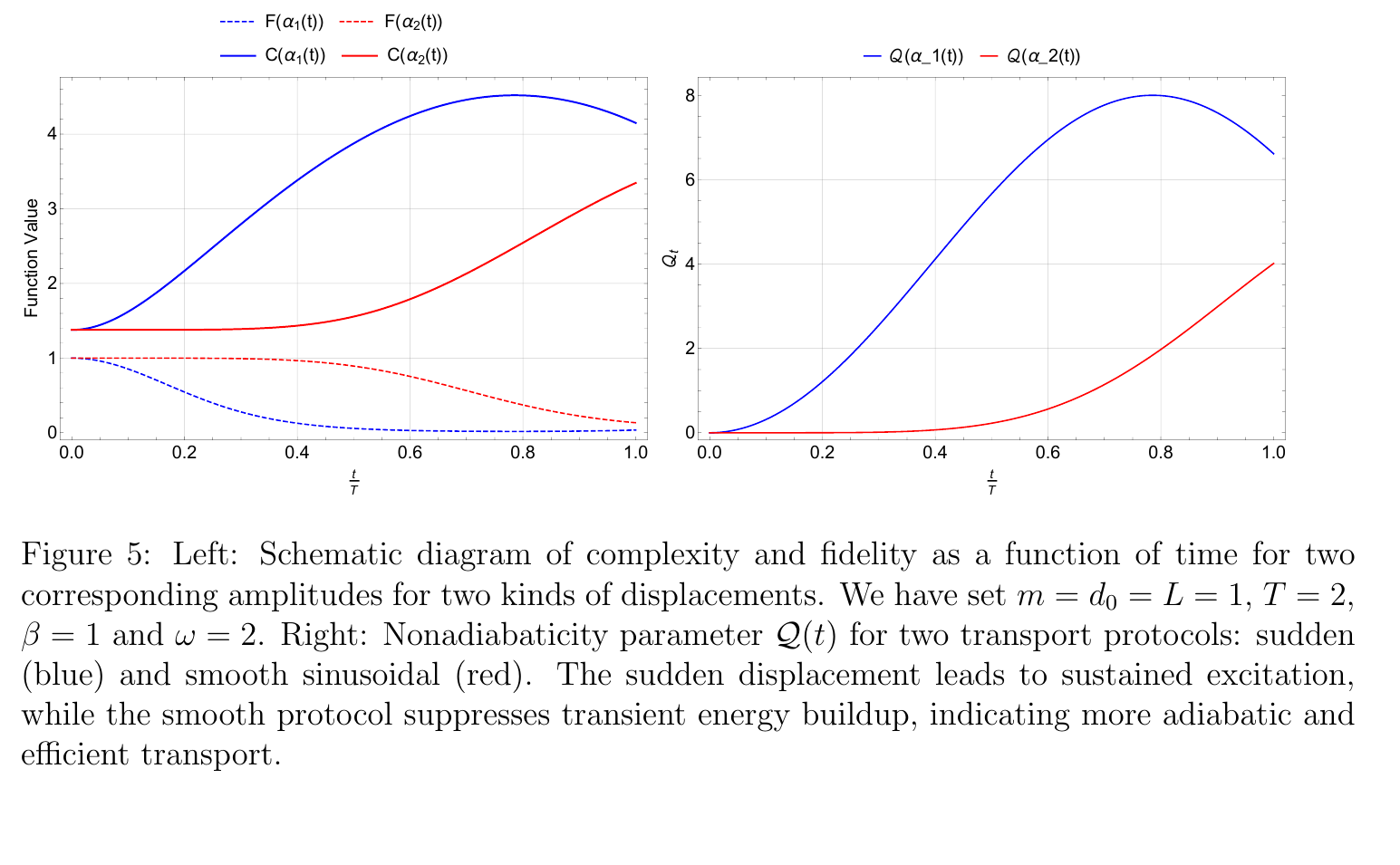
The left panel shows fidelity and complexity as functions of time. The sudden protocol causes fidelity to fall and complexity to grow strongly. The smooth protocol keeps the excitation smaller, so the fidelity remains higher and the complexity grows more gently.
The right panel shows $Q(t)$ for the two protocols. Since
\[Q(t)=2\lvert\alpha(t)\rvert^2,\]it directly tracks the excitation created by transport. The sudden protocol gives sustained excitation, while the smooth protocol gives smaller transient excitation.
The figure is therefore a visual summary of the central message: smooth control gives higher fidelity with lower complexity.
14. Reading Figure 6
Figure 6 studies how the complexity changes when the trap frequency $\omega$ is varied.
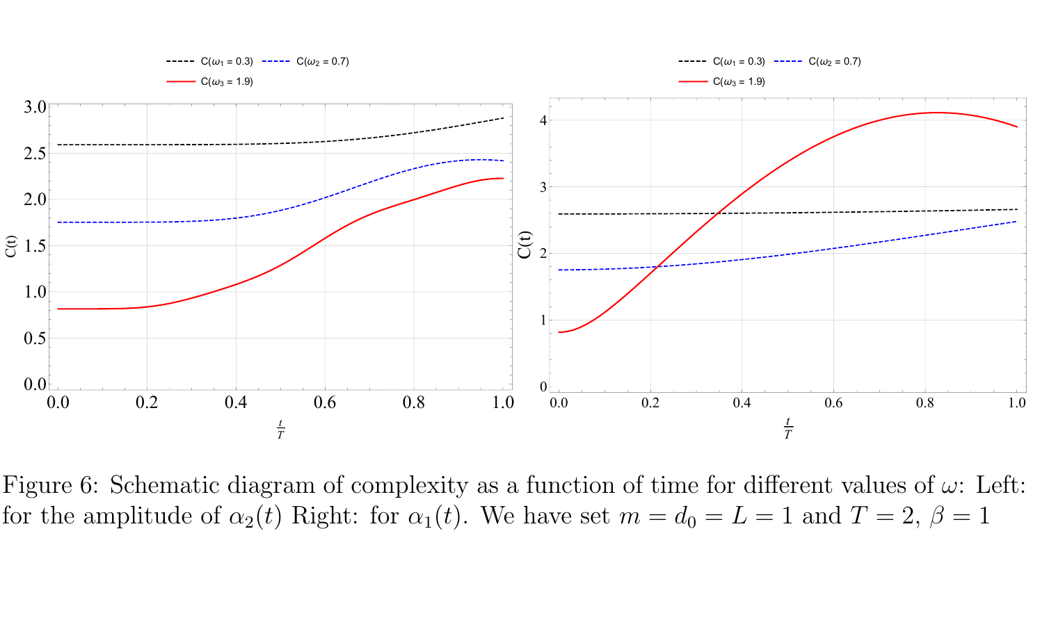
The frequency matters because the amplitude contains the phase factor $e^{i\omega t_1}$:
\[\int_0^t \dot d(t_1)e^{i\omega t_1}\,dt_1.\]This means the oscillator responds differently depending on how the protocol frequency content overlaps with the natural trap frequency.
The qualitative reading is:
| Frequency effect | Meaning |
|---|---|
| small $\omega$ | slower oscillator response |
| larger $\omega$ | stronger phase sensitivity |
| protocol near resonant response | larger displacement amplitude |
| larger $\lvert\alpha(t)\rvert$ | larger complexity |
Thus even for the same transport profile, changing $\omega$ changes the resource cost.
15. Connection With Adiabaticity
The word adiabatic means that the system has enough time to adjust to the changing Hamiltonian.
For the moving trap, adiabatic transport means $\dot d(t)$ is small and smooth. Nonadiabatic transport means $\dot d(t)$ is large, abrupt, or discontinuous.
The sudden protocol is nonadiabatic because it contains an impulse. The smooth sinusoidal protocol is closer to adiabatic because the velocity is finite and vanishes at the endpoints.
This connects directly with the earlier coupled-oscillator sections:
| Coupled-oscillator model | One-body transport model |
|---|---|
| weak mixing | smooth/adiabatic transport |
| strong mixing | sudden/nonadiabatic transport |
| low circuit depth | low displacement complexity |
| high circuit depth | high displacement complexity |
The models are different, but the organizing principle is the same.
16. Practical Control Principle
The section leads to a practical rule:
Smooth control fields reduce nonadiabatic excitation, and this simultaneously improves fidelity and lowers complexity.
For experiments, this means that the time profile of the control field is not a minor technical detail. It is part of the quantum resource budget.
If a protocol has sharp jumps, it injects energy into the system. That energy appears as:
- reduced fidelity,
- increased nonadiabaticity,
- increased complexity.
If a protocol is smooth, the state follows the moving trap more closely. Then the same transport task can be done with lower operational cost.
17. Compact Summary
The whole section can be compressed into one chain:
\[d(t) \longrightarrow \dot d(t) \longrightarrow \alpha(t) \longrightarrow \bigl(F(t),\mathcal C(t),Q(t)\bigr).\]The trap trajectory determines the trap velocity. The velocity determines the coherent displacement amplitude. The amplitude determines fidelity, complexity, and nonadiabaticity.
The best protocol is therefore not merely the fastest one. It is the one that moves the state while keeping $\lvert\alpha(t)\rvert^2$ small.
That is the key message of Section 4:
Temporal smoothness is a resource for high-fidelity, low-complexity quantum control.
The series closes with the final conclusion, where the coupled-oscillator and one-body transport lessons are collected into one picture.
Discussion