Contour Integration
The basic idea of contour integration is to extend the concept of integration from the real line to the complex plane. Instead of integrating a function along a real interval, we integrate it along a path (or contour) in the complex plane. This allows us to use the properties of analytic functions and the residues of poles to evaluate integrals that would be difficult or impossible to compute using standard real analysis techniques.
Cauchy-Riemann Conditions
Having introduced complex functions of a complex variable, we now discuss how to differentiate them. The derivative of a complex function $ f(z) $, similar to that of a real function, is defined as
\[\lim_{\delta z \to 0} \frac{f(z+\delta z)-f(z)}{(z+\delta z)-z} = \lim_{\delta z \to 0} \frac{\delta f}{\delta z} = \frac{df}{dz} = f'(z),\]provided that this limit is independent of the direction from which $ \delta z $ approaches zero.
For real-valued functions, the derivative exists at a point if the right-hand and left-hand limits are equal. In the complex plane, however, the variable $ z $ can approach a point from infinitely many directions. Hence, requiring the limit to be the same in all directions is a much stronger condition.
Let the complex variable be written as
\[z = x + iy,\]where $ x $ and $ y $ are real variables. Small changes in $ x $ and $ y $ produce a change in $ z $ given by
\[\delta z = \delta x + i\,\delta y .\]If
\[f(z) = u(x,y) + i\,v(x,y),\]then the corresponding change in the function is
\[\delta f = \delta u + i\,\delta v .\]Hence,
\[\frac{\delta f}{\delta z} = \frac{\delta u + i\,\delta v}{\delta x + i\,\delta y}.\]To understand the restriction imposed by the derivative, we evaluate the limit along two different paths (as shown in Fig. 6.4).
First approach:
Let $ \delta y = 0 $ and allow $ \delta x \to 0 $. Then
assuming the partial derivatives exist.
Second approach:
Let $ \delta x = 0 $ and allow $ \delta y \to 0 $. This gives
For the derivative $ df/dz $ to exist, both limits must be equal. By equating the real and imaginary parts, we obtain
\[\color{Brown}{ \boxed{ \frac{\partial u}{\partial x} = \frac{\partial v}{\partial y}, \qquad \frac{\partial u}{\partial y} = -\,\frac{\partial v}{\partial x} }}\]These equations are known as the Cauchy–Riemann conditions. They play a fundamental role in complex analysis.
The Cauchy–Riemann conditions are necessary for the derivative of $ f(z) $ to exist. Moreover, if these conditions are satisfied and the partial derivatives of $ u(x,y) $ and $ v(x,y) $ are continuous, then the derivative $ df/dz $ does exist.
This can be seen by expressing the change in $ f $ as
\[\delta f = \left( \frac{\partial u}{\partial x} + i\,\frac{\partial v}{\partial x} \right)\delta x + \left( \frac{\partial u}{\partial y} + i\,\frac{\partial v}{\partial y} \right)\delta y .\]Analytic functions are those that are complex differentiable at every point in their domain. Examples include polynomials, exponential functions, and trigonometric functions.
Example of an analytic function
Consider the function
\[f(z) = z^{2}.\]Writing $ z = x + iy $, we obtain
\[f(z) = (x + iy)^{2} = (x^{2} - y^{2}) + i(2xy).\]Hence, the real and imaginary parts are
\[u(x,y) = x^{2} - y^{2}, \qquad v(x,y) = 2xy.\]Using the Cauchy–Riemann conditions,
\[\frac{\partial u}{\partial x} = 2x = \frac{\partial v}{\partial y}, \qquad \frac{\partial u}{\partial y} = -2y = -\,\frac{\partial v}{\partial x}.\]Thus, the Cauchy–Riemann conditions are satisfied everywhere in the complex plane. Since all the partial derivatives are continuous, we conclude that $ f(z) = z^{2} $ is an analytic function.
Example of a non-analytic function
Now consider the function
\[f(z) = z^{*},\]where $ z^{*} $ denotes the complex conjugate of $ z $. Writing $ z = x + iy $, we have
\[f(z) = x - iy,\]so that
\[u(x,y) = x, \qquad v(x,y) = -y.\]Applying the Cauchy–Riemann conditions,
\[\frac{\partial u}{\partial x} = 1, \qquad \frac{\partial v}{\partial y} = -1.\]Since these quantities are not equal, the Cauchy–Riemann conditions are not satisfied. Therefore, $ f(z) = z^{*} $ is not analytic.
It is worth noting that $ f(z) = z^{*} $ is continuous everywhere in the complex plane, yet it is nowhere differentiable as a complex function. This highlights an important difference between real and complex analysis. In real-variable calculus, the derivative is mainly a local property, describing the behavior of a function near a point. In contrast, the existence of a derivative for a complex function has much stronger consequences.
For an analytic function, the real and imaginary parts each satisfy Laplace’s equation, and the function possesses derivatives of all orders. Thus, in complex analysis, the derivative not only determines the local behavior of a function but also strongly influences its global behavior.
Cauchy’s Integral Theorem
Cauchy’s Integral Theorem states that if a function is analytic (holomorphic) within and on a closed contour, then the integral of the function around that contour is zero:
\[\color{Red}{ \boxed{\oint_C f(z) \, dz = 0 }}\]where $ C $ is a closed contour in the complex plane.
Contour Integrals
The integral of a complex function over a contour in the complex plane is defined in close analogy with the Riemann integral of a real function along the real axis. Consider a contour joining two points $z_0$ and $z_0’$. Divide the contour into $n$ small segments by selecting intermediate points
\[z_0, z_1, z_2, \ldots, z_n=z_0'.\]On each segment choose an arbitrary point $\zeta_j$ between $z_{j-1}$ and $z_j$. We then form the sum
\[S_n=\sum_{j=1}^{n} f(\zeta_j)\,(z_j-z_{j-1}).\]If, in the limit $n\to\infty$, the maximum segment length $|z_j-z_{j-1}|\to 0$ and the limit of $S_n$ exists independently of how the points $z_j$ and $\zeta_j$ are chosen, this limit defines the contour integral
\[\int_{z_0}^{z_0'} f(z)\,dz .\]A particularly important case occurs when the contour is closed, that is, when the initial and final points coincide. For a function that possesses an antiderivative (is analytic in the region enclosed by the contour), the contour integral over any closed path vanishes. The reason is that the integral depends only on the endpoints of the path; when these coincide, the net contribution must be zero. This property underlies many results of complex analysis and is a special case of Cauchy’s integral theorem.
As an illustration, consider integrating $z^n$ around a rectangle with corners $z_1, z_2, z_3, z_4$, traversed in sequence and returning to $z_1$. For $n\neq -1$,
\[\int z^n\,dz =\frac{z^{n+1}}{n+1}\Biggr|_{z_1}^{z_2} +\frac{z^{n+1}}{n+1}\Biggr|_{z_2}^{z_3} +\frac{z^{n+1}}{n+1}\Biggr|_{z_3}^{z_4} +\frac{z^{n+1}}{n+1}\Biggr|_{z_4}^{z_1}.\]Each corner point appears once as an upper limit and once as a lower limit, so all contributions cancel. Hence,
\[\oint z^n\,dz=0 \qquad (n\neq -1).\]Cauchy’s Integral Formula
As in the preceding section, consider a function $f(z)$ that is analytic on and within a closed contour $C$. We wish to prove the fundamental result
\[\boxed{\frac{1}{2\pi i}\oint_C \frac{f(z)}{z-z_0}\,dz=f(z_0),}\]where $z_0$ is any point lying in the interior of the region bounded by $C$. This is the second of the two basic theorems introduced in Section 6.3. Since $z$ lies on the contour $C$ while $z_0$ is strictly inside it, we always have $z-z_0\neq 0$, so the integral is well defined. Although $f(z)$ itself is analytic, the integrand $f(z)/(z-z_0)$ is not analytic at $z=z_0$ unless $f(z_0)=0$.
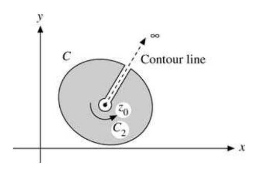
Deforming the contour as illustrated in figure above, the original contour $C$ is replaced by a new contour consisting of an outer contour and a small circle $C_2$ enclosing the point $z_0$. Since the integrand is analytic everywhere between these two contours, we have
\[\oint_C \frac{f(z)}{z-z_0}\,dz-\oint_{C_2} \frac{f(z)}{z-z_0}\,dz=0 .\]Parameterizing the small circle by $z=z_0+r e^{i\theta}$, with $r$ small and traversed counterclockwise, gives
\[\oint_{C_2} \frac{f(z)}{z-z_0}\,dz =\oint_{C_2} \frac{f(z_0+r e^{i\theta})}{r e^{i\theta}}\, i r e^{i\theta}\,d\theta .\]Taking the limit $r\to 0$ and using the continuity of $f(z)$ at $z=z_0$, we obtain
\[\oint_{C_2} \frac{f(z)}{z-z_0}\,dz =i f(z_0)\int_{0}^{2\pi} d\theta =2\pi i\, f(z_0),\]which establishes the Cauchy integral formula.
This result is remarkable: the value of an analytic function at any interior point $z_0$ is completely determined by its values on the boundary contour $C$. The situation is closely analogous to Gauss’s law in two dimensions, where an interior charge is determined by a surface integral over the boundary, or to the determination of a function via Green’s functions in boundary-value problems such as Kirchhoff diffraction theory. If, however, the point $z_0$ lies outside the contour $C$, then the integrand is analytic everywhere on and within $C$, and Cauchy’s integral theorem implies that the integral vanishes. Thus,
\[\frac{1}{2\pi i}\oint_C \frac{f(z)}{z-z_0}\,dz= \begin{cases} f(z_0), & z_0 \text{ interior to } C,\\ 0, & z_0 \text{ exterior to } C . \end{cases}\]Residue Theorem
If the Laurent expansion of a function
\[f(z)=\sum_{n=-\infty}^{\infty} a_n (z-z_0)^n\]is integrated term by term around a closed contour that encircles one isolated singular point $z_0$ once in the counterclockwise sense, we obtain
\[a_n \oint (z-z_0)^n \, dz = a_n \frac{(z-z_0)^{n+1}}{n+1}\biggr|_{z_1}^{z_1} =0, \qquad n\neq -1 . \tag{1}\]However, if $n=-1$,
\[a_{-1} \oint (z-z_0)^{-1} \, dz = a_{-1} \oint \frac{i r e^{i\theta}\, d\theta}{r e^{i\theta}} = 2\pi i\, a_{-1}. \tag{2}\]Thus,
\[\frac{1}{2\pi i}\oint f(z)\, dz = a_{-1}. \tag{3}\]The constant $a_{-1}$, the coefficient of $(z-z_0)^{-1}$ in the Laurent expansion, is called the residue of $f(z)$ at $z=z_0$.
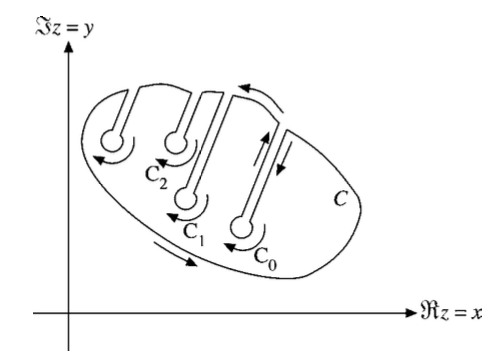
A set of isolated singularities can be handled by deforming the contour as shown in figure below. Cauchy’s integral theorem leads to
\[\oint_C f(z)\, dz +\oint_{C_0} f(z)\, dz +\oint_{C_1} f(z)\, dz +\oint_{C_2} f(z)\, dz +\cdots = 0 . \tag{4}\]The circular integral around any given singular point is given by Eq. (3),
\[\oint_{C_i} f(z)\, dz = -2\pi i\, a_{-1,z_i}, \tag{5}\]assuming a Laurent expansion about the singular point $z=z_i$. The negative sign arises from the clockwise sense of integration, as shown in figure below.
Combining Eqs. (4) and (5), we obtain
\[\boxed{ \oint_C f(z)\, dz = 2\pi i \left(a_{-1,z_0}+a_{-1,z_1}+a_{-1,z_2}+\cdots\right) = 2\pi i \times (\text{sum of enclosed residues}) }\]This result is known as the residue theorem. The problem of evaluating one or more contour integrals is thereby reduced to the algebraic problem of computing the residues at the enclosed singular points.
It states that if $ f(z) $ is analytic in a region except for isolated singularities (poles), then the integral of $ f(z) $ around a closed contour $ C $ that encloses these singularities is given by:
\[\oint_C f(z) \, dz = 2\pi i \sum \text{Res}(f, a_k)\]where the sum is over all singularities $ a_k $ inside the contour $ C $, and $ \text{Res}(f, a_k) $ is the residue of $ f $ at the singularity $ a_k $.
Integrals in Quantum Mechanics
Integral of a Lorentzian Function:
\[\int_{-\infty}^{\infty} \frac{1}{(p^2 + \alpha^2)} \, dp = \frac{\pi}{\alpha}\]Integral of a Power Function in Momentum Space:
\[\int_{-\infty}^{\infty} \frac{p^n}{(p^2 + \beta^2)} \, dp = 0 \quad \text{for odd } n\]Integral of a Gaussian Function in Momentum Space:
\[\int_{-\infty}^{\infty} e^{-\beta p^2} \, dp = \sqrt{\frac{\pi}{\beta}}\]Integral of an Exponential Function in Momentum Space:
\[\int_{-\infty}^{\infty} e^{ipx/\hbar} \, dp = 2\pi \hbar \delta(x)\]Integral of a Rational Function with Exponential in Momentum Space:
\[\int_{-\infty}^{\infty} \frac{e^{ipx/\hbar}}{(p^2 + \alpha^2)} \, dp = \frac{\pi}{\alpha} e^{-\alpha |x|/\hbar}\]Integral of Cosine Function over a Rational Function:
\[\int_{-\infty}^{\infty} \frac{\cos(ax)}{x^2 + b^2} \, dx = \frac{\pi}{b} e^{-b|a|}\]Integral of Sine Function over a Rational Function:
\[\int_{-\infty}^{\infty} \frac{\sin(ax)}{x^2 + b^2} \, dx = \pi \frac{\text{sgn}(a)}{b} e^{-b|a|}\]where $\text{sgn}(a)$ is the sign function and equals 1 for $ a > 0 $, -1 for $ a < 0 $, and 0 for $ a = 0 $.
Some special integrals
Integral of Sine Function over a Rational Function:
\[\int_{-\infty}^{\infty} \frac{\sin(ax)}{x} \, dx = \pi \text{sgn}(a)\]where $ \text{sgn}(a) $ is the sign function and equals 1 for $ a > 0 $, -1 for $ a < 0 $, and 0 for $ a = 0 $.
\[\int_{0}^{\infty} \frac{\sin(x)}{x} \, dx = \frac{\pi}{2}\]Integral of a Logarithmic Function:
\[\int_{0}^{\infty} \frac{\ln(x)}{x^2 + 1} \, dx = 0\]Integral of a Power Function:
\[\int_{0}^{\infty} \frac{x^{m-1}}{x^2 + 1} \, dx = \frac{\pi}{2} \csc\left(\frac{m\pi}{2}\right) \quad (0 < m < 2)\]Integral of a Hyperbolic Function:
\[\int_{-\infty}^{\infty} \frac{1}{\cosh(x)} \, dx = \pi\]Integral of a Complex Exponential Function:
\[\int_{-\infty}^{\infty} e^{ix^2} \, dx = \sqrt{\frac{\pi}{2}} (1 + i)\]Application: Evaluation of a Real Integral Using Contour Integration
Contour integration can be used to evaluate certain real integrals by extending them into the complex plane. Consider the integral
\[I=\int_{-\infty}^{\infty}\frac{e^{ix}}{x^2+1}\,dx .\]Step 1: Define the Complex Function
We associate the given real integral with the complex function
\[f(z)=\frac{e^{iz}}{z^2+1},\]which has simple poles at
\[z=\pm i .\]Step 2: Choice of Contour
Since
\[e^{iz}=e^{i(x+iy)}=e^{ix-y},\]the exponential term decays exponentially in the upper half-plane ($y>0$).
Hence, we close the contour with a semicircle of radius $R$ in the upper half-plane.
By Jordan’s lemma, the contribution from the semicircular arc vanishes as $R\to\infty$.
Step 3: Singularities Inside the Contour
Only one singularity lies inside the upper half-plane:
\[z=i .\]Step 4: Compute the Residue at $z=i$
The residue of $f(z)$ at $z=i$ is
\[\operatorname{Res}(f,z=i) =\lim_{z\to i}(z-i)\frac{e^{iz}}{(z-i)(z+i)} =\frac{e^{ii}}{2i} =\frac{e^{-1}}{2i}.\]Step 5: Apply the Residue Theorem
By the residue theorem,
\[\oint f(z)\,dz =2\pi i\,\operatorname{Res}(f,z=i) =2\pi i\cdot\frac{e^{-1}}{2i} =\pi e^{-1}.\]Since the contribution from the semicircular arc vanishes, the contour integral reduces to the original real integral. Therefore,
\[\int_{-\infty}^{\infty}\frac{e^{ix}}{x^2+1}\,dx=\pi e^{-1}.\]