By M. Lieber Received 18 June 1974

Schrodinger equation in momentum space is obtained by Fourier transforming the coordinate space equation. Lets consider the time-independent Schrodinger equation in one dimension in position space:

\[\frac{p^2}{2m} \Psi(x) + V(x) \Psi(x) = E \Psi(x) \tag{1}\]

or equivalently,

\[\left(E-\frac{p^2}{2m}\right) \Psi(x)= V(x) \Psi(x) \tag{2}\]

To transform this into momentum space, we take the Fourier transform of both sides. The Fourier transform of the wave function is given by:

\[\Phi(p) = \frac{1}{\sqrt{2\pi \hbar}} \int_{-\infty}^{\infty} \Psi(x) e^{-ipx/\hbar} dx\]

Applying the Fourier transform to (2), we have:

\[\begin{aligned} \frac{1}{\sqrt{2\pi \hbar}} \int_{-\infty}^{\infty} \left(E-\frac{p^2}{2m}\right) \Psi(x) e^{-ipx/\hbar} dx &= \frac{1}{\sqrt{2\pi \hbar}} \int_{-\infty}^{\infty} V(x) \Psi(x) e^{-ipx/\hbar} dx\\ \left(E-\frac{p^2}{2m}\right) \phi(p) &= \frac{1}{\sqrt{2\pi \hbar}} \int_{-\infty}^{\infty} \tilde{V}(p-p') \phi(p') dp' \end{aligned}\tag{3}\]

where $ \tilde{V}(p-p’) $ is the Fourier transform of the potential $ V(x) $:

\[\tilde{V}(p) = \frac{1}{\sqrt{2\pi \hbar}} \int_{-\infty}^{\infty} V(x) e^{-ipx/\hbar} dx\]

Thus, the Schrodinger equation in momentum space becomes:

\[\color{brown}{\boxed{ \left(E-\frac{p^2}{2m}\right) \phi(p) = \frac{1}{\sqrt{2\pi \hbar}} \int_{-\infty}^{\infty} \tilde{V}(p-p') \phi(p') dp' }} \tag{4}\]

Consider potential $V(x) = V_0 \delta(x)$

For the delta function potential, the Fourier transform is:

\[\tilde{V}(p) = \frac{V_0}{\sqrt{2\pi \hbar}}\]

Substituting this into (4), we get:

\[\left(E-\frac{p^2}{2m}\right) \phi(p) = \frac{V_0}{2\pi \hbar} \int_{-\infty}^{\infty} \phi(p') dp' \tag{5}\]

Let $ C = \int_{-\infty}^{\infty} \phi(p’) dp’ $. Then (5) becomes:

\[\left(E-\frac{p^2}{2m}\right) \phi(p) = \frac{V_0}{2\pi \hbar} C \tag{6}\]

Rearranging (6), we have:

\[\phi(p) = \frac{V_0 C}{2\pi \hbar \left(E-\frac{p^2}{2m}\right)} \tag{7}\]

To find $ C $, we integrate both sides of (7) over all $ p $:

\[C = \int_{-\infty}^{\infty} \phi(p) dp = \frac{V_0 C}{2\pi \hbar} \int_{-\infty}^{\infty} \frac{dp}{E-\frac{p^2}{2m}} \tag{8}\]

The integral on the right side can be evaluated using contour integration techniques. The result is:

\[\int_{-\infty}^{\infty} \frac{dp}{E-\frac{p^2}{2m}} = -\pi \sqrt{\frac{2m}{-E}} \quad \text{for } E < 0\]

Substituting this back into (8), we get:

\[C = \frac{V_0 C}{2\pi \hbar} \left(-\pi \sqrt{\frac{2m}{-E}}\right)\]

This leads to the condition for non-trivial solutions (i.e., $ C \neq 0 $):

\[1 = -\frac{V_0}{2\hbar} \sqrt{\frac{2m}{-E}}\]

Solving for $ E $, we find the bound state energy:

\[E = -\frac{m V_0^2}{2 \hbar^2} \tag{9}\]

Thus, the bound state energy for a particle in a delta function potential well is given by (9). The corresponding momentum space wave function can be obtained from (7) using the value of $ E $ found above.

\[\color{brown}{\boxed{ E = -\frac{m V_0^2}{2 \hbar^2} }}\]

Putting eqn (9) back into (7) gives the momentum space wave function for the bound state.

\[\phi(p) = -\frac{mV_0 C}{\pi \hbar \left(\frac{m^2 V_0^2}{ \hbar^2}+p^2\right)}\]

Upon normalization, we can determine the constant $ C $ which comes out to be:

\[C = -\frac{m V_0 \sqrt{\frac{2 \pi\hbar}{m V_0}}}{\hbar }\]

Therefore, the normalized momentum space wave function is:

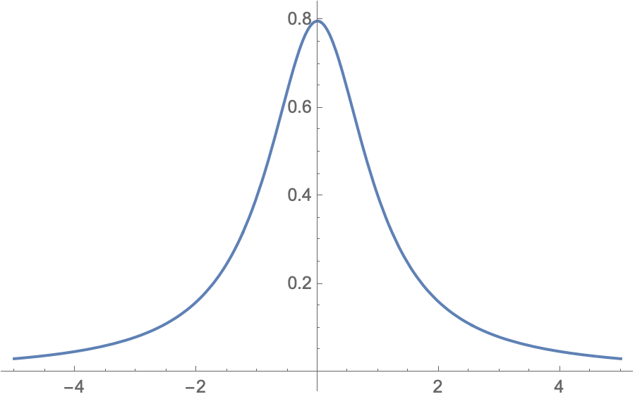
\[\phi(p) = \sqrt{\frac{2}{\pi}} \left(\frac{m V_0}{\hbar}\right)^{3/2}\frac{1}{\left[\left(\frac{m V_0}{ \hbar}\right)^2+p^2\right]}\]

The plot of the momentum space wave function is shown below with respect to momentum p.

The coordinate space wave function can be obtained by inverse Fourier transforming the momentum space wave function. Here contour integration can be used to evaluate the integral as the case for positve and negative x can be treated separately. The final result for the coordinate space wave function is:

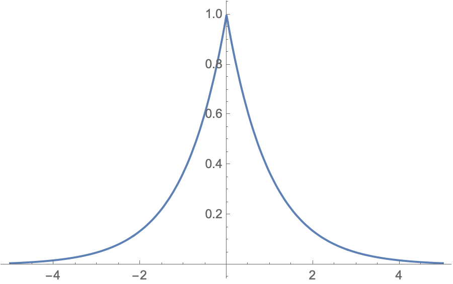
\[\Psi(x) = \sqrt{\frac{m V_0}{\hbar^2}} e^{-\frac{m V_0}{\hbar^2}|x|}\]

Note $V_0$ is a positive quantity here representing the depth of the potential well. The plot of the coordinate space wave function is shown below with respect to position x.

This completes the solution of the Schrodinger equation in momentum space for a delta function potential well, yielding both the bound state energy and the corresponding wave functions in momentum and coordinate space.

Scattering Problem

For scattering states with positive energy $ E > 0 $, we can analyze the scattering problem using the momentum space Schrodinger equation (4). Consider an incident plane wave with momentum $ p_0 = \sqrt{2mE} $ with scattering from the delta function potential as given in the previous section.

\[\left(E-\frac{p^2}{2m}\right) \phi(p) = \frac{V_0}{2\pi \hbar} \int_{-\infty}^{\infty} \phi(p') dp' \tag{10}\]

Let $E= \frac{p_0^2}{2m}$ and $\alpha=\frac{mV_0}{\pi \hbar}C$, where $C$ is the integral on the right side $ C = \int_{-\infty}^{\infty} \phi(p’) dp’ $. Then (10) becomes:

\[\left(p_0^2-p^2\right) \phi(p) = \alpha\tag{11}\]

The denominator $p_0^2-p^2$ vanishes at $p=\pm p_0$. Hence $\phi(p)$ is singular on the real axis, and its integral

\[C=\int_{-\infty}^{\infty}\phi(p)\,dp\]

is not an ordinary Riemann integral. Further, this case is distinct from the bound state case treated earlier as there were no singularities on the real axis do the negative energy. The most general solution for $\phi(p)$ must therefore include delta functions at the singular points to account for the incident and reflected waves in the scattering process.

Why the principal value alone is not enough

If you only define

\[(p_0^2-p^2)^{-1} \;\to\; P[(p_0^2-p^2)^{-1}],\]

you get one particular solution, but not the most general solution.

In distribution theory:

Whenever a coefficient multiplying $\phi(p)$ vanishes at some points, delta functions supported at those points may appear in the solution.

Here, since

\[(p_0^2-p^2)\,\delta(p\mp p_0)=0,\]

delta functions at $p=\pm p_0$ solve the homogeneous equation.

Homogeneous vs particular solutions

(a) Homogeneous solutions

Consider

\[(p_0^2-p^2)\,\phi(p)=0\]

This is satisfied by

\[\boxed{ \delta(p-p_0),\qquad \delta(p+p_0) }\]

because multiplication by $p_0^2-p^2$ annihilates them.

These correspond physically to free incoming and outgoing momentum eigenstates.

(b) Particular solution

A particular solution of

\[(p_0^2-p^2)\,\phi(p)=\text{constant}\]

is

\[\phi(p)=\alpha\,P[(p_0^2-p^2)^{-1}]\]

This is the scattered (off-shell) contribution.

Combining homogeneous + particular solutions gives

\[\boxed{ \phi(p) = A\,\delta(p-p_0) + B\,\delta(p+p_0) + \alpha\,P[(p_0^2-p^2)^{-1}] } \tag{12}\]

where $A,B$ are constants representing the amplitudes of the incident and reflected waves, respectively. Integrating (30) over all $p$ gives

\[\alpha\;\frac{\pi\hbar}{mV_0} = A + B + \alpha \int_{-\infty}^{\infty} P[(p_0^2-p^2)^{-1}]\,dp\]

But

\[\int_{-\infty}^{\infty} P[(p_0^2-p^2)^{-1}]\,dp = 0\]

(by symmetry of the principal value).

Therefore:

\[\boxed{ \alpha=\frac{m V_0}{\pi\hbar}(A+B) } \tag{13}\]

Now the general solution must be the sum of incident plane waves and scattered waves, i.e.,

\[\phi(p) = \delta(p - p_0) + f(p) \{2m P (p_0^2 - p^2)^{-1}-\frac{im\pi}{p_0}\left(\delta(p - p_0)+\delta(p + p_0)\right) \} \tag{14}\]

where $ f(p) $ is the scattering amplitude. Comparing (12) and (14), we can identify the coefficients $ A $ and $ B $ in terms of the scattering amplitude $ f(p) $. Comparing the principal value terms in both expressions, we have:

\[\frac{m V_0}{\pi \hbar }(A+B)=\alpha = 2m f(p) \tag{15}\]

Next, comparing the delta function coefficients, we have:

\[A = 1 - \frac{im\pi}{p_0} f(p) \tag{16}\] \[B = - \frac{im\pi}{p_0} f(p) \tag{17}\]

Now substituting (15) into (16) and (17), we can solve for the scattering amplitude $ f(p) $ as:

\[f(p) = \frac{\frac{V_0}{2\pi \hbar}}{1 + i \frac{m V_0}{p_0\hbar}} \tag{18}\]

Thus, the scattering amplitude for a particle scattering off a delta function potential in momentum space is given by (18). Thus our final expression for the momentum space wave function from (14) becomes:

\[\phi(p) = \delta(p - p_0) + \frac{\frac{V_0}{2\pi \hbar}}{1 + i \frac{m V_0}{p_0\hbar}} \left\{2m P (p_0^2 - p^2)^{-1}-\frac{im\pi}{p_0}\left(\delta(p - p_0)+\delta(p + p_0)\right) \right\}\]

---

Contour integration techniques\

Given an wave function in momentum space of the form:

\[\phi(p) = \frac{A}{(p^2 + \alpha^2)}\]

To find the corresponding coordinate space wave function, we perform the inverse Fourier transform:

\[\Psi(x) = \frac{1}{\sqrt{2\pi \hbar}} \int_{-\infty}^{\infty} \phi(p) e^{ipx/\hbar} dp = \frac{A}{\sqrt{2\pi \hbar}} \int_{-\infty}^{\infty} \frac{e^{ipx/\hbar}}{(p^2 + \alpha^2)} dp\]

To evaluate this integral, we can use contour integration techniques from complex analysis. The integrand has poles at $ p = i\alpha $ and $ p = -i\alpha $. Depending on the sign of $ x $, we will close the contour in the upper or lower half-plane.

1. Case 1: $ x > 0 $ For $ x > 0 $, we close the contour in the upper half-plane. The only pole inside this contour is at $ p = i\alpha $. Using the residue theorem, we calculate the residue at this pole:

   \[\text{Res}\left(\frac{e^{ipx/\hbar}}{p^2 + \alpha^2}, p = i\alpha\right) = \lim_{p \to i\alpha} (p - i\alpha) \frac{e^{ipx/\hbar}}{(p - i\alpha)(p + i\alpha)} = \frac{e^{i(i\alpha)x/\hbar}}{2i\alpha} = \frac{e^{-\alpha x/\hbar}}{2i\alpha}\]

   Applying the residue theorem, we have:

   \[\int_{-\infty}^{\infty} \frac{e^{ipx/\hbar}}{(p^2 + \alpha^2)} dp = 2\pi i \cdot \text{Res} = 2\pi i \cdot \frac{e^{-\alpha x/\hbar}}{2i\alpha} = \frac{\pi e^{-\alpha x/\hbar}}{\alpha}\]

   Thus, for $ x > 0 $:

   \[\Psi(x) = \frac{A}{\sqrt{2\pi \hbar}} \cdot \frac{\pi e^{-\alpha x/\hbar}}{\alpha} = \frac{A \sqrt{\pi}}{\alpha \sqrt{2\hbar}} e^{-\alpha x/\hbar}\]

2. Case 2: $ x < 0 $

   For $ x < 0 $, we close the contour in the lower half-plane. The only pole inside this contour is at $ p = -i\alpha $. Calculating the residue at this pole:

   \[\text{Res}\left(\frac{e^{ipx/\hbar}}{p^2 + \alpha^2}, p = -i\alpha\right) = \lim_{p \to -i\alpha} (p + i\alpha) \frac{e^{ipx/\hbar}}{(p - i\alpha)(p + i\alpha)} = \frac{e^{i(-i\alpha)x/\hbar}}{-2i\alpha} = \frac{e^{\alpha x/\hbar}}{-2i\alpha}\]

   Applying the residue theorem, we have:

   \[\int_{-\infty}^{\infty} \frac{e^{ipx/\hbar}}{(p^2 + \alpha^2)} dp = 2\pi i \cdot \text{Res} = 2\pi i \cdot \frac{e^{\alpha x/\hbar}}{-2i\alpha} = -\frac{\pi e^{\alpha x/\hbar}}{\alpha}\]

   Thus, for $ x < 0 $:

   \[\Psi(x) = \frac{A}{\sqrt{2\pi \hbar}} \cdot \left(-\frac{\pi e^{\alpha x/\hbar}}{\alpha}\right) = -\frac{A \sqrt{\pi}}{\alpha \sqrt{2\hbar}} e^{\alpha x/\hbar}\]

   Combining both cases, we can write the coordinate space wave function as:

   \[\Psi(x) = \frac{A \sqrt{\pi}}{\alpha \sqrt{2\hbar}} e^{-\alpha |x|/\hbar}\]

   This result shows that the coordinate space wave function decays exponentially with distance from the origin, consistent with the expected behavior for a bound state in a potential well.