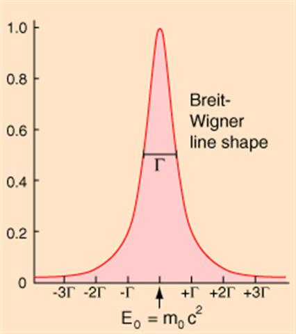
In this lecture, we will start by revisiting the basics of quantum scattering, focusing on partial wave analysis and phase shifts. The graph at the top illustrates the Breit-Wigner resonance curve, which we will discuss in detail after exploring resonance scattering and its role in energy-dependent cross-sections.

Scattering Cross-Section

The one-dimensional Schrödinger equation for a particle of mass $m$ in a potential $V(x)$ is:

\[-\frac{\hbar^2}{2m} \frac{d^2\psi}{dx^2} + V(x)\psi = E\psi.\]

The general solution is:

\[\psi(x) = \begin{cases} Ae^{ikx} + Be^{-ikx}, & E > V \ (\text{plane waves}), \\ C e^{-\lambda x}, & E < V \ (\text{exponential decay}), \end{cases}\]

where $k = \sqrt{2m(E - V) / \hbar^2}$ and $\lambda = \sqrt{2m(V - E) / \hbar^2}$.

Bound States

Bound states occur for $E < V$, where wavefunctions decay exponentially:

\[\psi(x) \sim e^{-\lambda |x|}, \quad E = V - \frac{\hbar^2 \lambda^2}{2m}.\]

Such states have discrete energy levels, a hallmark of quantum systems.

Scattering States

Scattering states arise when $E > V$, allowing free motion:

\[\psi(x) \sim e^{\pm ikx}.\]

The energy relation is $E = V + \frac{\hbar^2 k^2}{2m}$.

Scattering Cross-Section

For the scattering potential $V(\mathbf{x})$, the total wavefunction at point $p$ is sum of plane wave and spherical wave modulated by factor $f$ due to scattering and is given by:

\[\psi(\mathbf{x}) = e^{i\mathbf{k \cdot x}} + f(\mathbf{k',k}) \frac{e^{ikr}}{r}, \text{and}\;r=|\mathbf{x}|\]

where $f(\mathbf{k’,k})$ is the scattering amplitude:

\[f(\mathbf{k',k}) = -\frac{1}{4\pi} \int d^3x' e^{-i\mathbf{k' \cdot x'}} V(\mathbf{x'}) \psi(\mathbf{x'}).\]

The differential cross-section is:

\[\frac{d\sigma}{d\Omega} = |f(\mathbf{k',k})|^2.\]

The total cross-section integrates over all angles:

\[\sigma_{\text{total}} = \int \frac{d\sigma}{d\Omega} \, d\Omega.\]

Partial Wave Analysis

Expanding the incident wave in spherical harmonics $Y_{lm}(\theta, \phi)$:

\[\phi(\mathbf{x}) = e^{i\mathbf{k \cdot x}} = \sum_{l=0}^\infty (2l+1) i^l j_l(kr) P_l(\cos\theta).\]

The differential cross-section becomes:

\[\frac{d\sigma}{d\Omega} = \left| \frac{1}{k} \sum_{l=0}^\infty (2l+1) e^{i\delta_l} \sin\delta_l P_l(\cos\theta) \right|^2.\]

Here, $\delta_l$ are phase shifts from scattering.

---

Nuclear Reactions: Revisited

Here, we introduce Direct and Compound nuclear reactions to contrast them with Resonance Reactions, which serve as an intermediate between the two.

1. Direct Reactions

Direct reactions occur when the incident particle interacts with the nucleus over a short time, leading to a direct transition between nuclear states. These reactions are characterized by their fast nature and relatively low probability of occurrence.

Key Features

• Short interaction time: The process occurs quickly, typically within $10^{-22}$ seconds.
• Small energy transfer: The incident particle imparts minimal energy to the nucleus.
• Types of direct reactions: Elastic scattering, inelastic scattering, transfer reactions, and knockout reactions.

---

2. Compound Nucleus Reactions

Compound nucleus reactions occur when the incident particle is fully absorbed by the target nucleus, forming an intermediate, highly excited state. This intermediate state, known as the compound nucleus, subsequently decays into a final configuration.

Key Features

• Formation: The compound nucleus is a short-lived, highly excited state, existing for a relatively long timescale ($10^{-16}$ to $10^{-14}$ seconds) compared to direct reactions.
• Statistical nature: The decay channels exhibit a statistical distribution as the compound nucleus loses all memory of the entrance channel’s specific properties.
  • Decay mechanism: The decay of the compound nucleus mimics evaporation, where the emitted particle behaves like a droplet evaporating from a heated liquid. The energy distribution of the emitted particles reflects the thermal excitation of the compound nucleus.
  • Angular distribution: The angular distribution of emitted particles is typically flat, reflecting the random nature of the decay process and the lack of memory of the entrance channel’s directionality.
  • Two-step process: The formation and decay of the compound nucleus are independent processes. The compound nucleus achieves equilibrium before decaying, and the final state is uncorrelated with the entrance channel parameters.

---

3. Resonance Reactions

Resonance reactions lie between the extremes of direct reactions and compound nucleus reactions. They involve discrete, quasibound nuclear states in the energy spectrum.

• Resonance states: Quasibound states with lifetimes long enough to form distinct energy levels, but still unstable against decay.
• High cross-section: Resonances exhibit a significantly increased probability of interaction at specific energies.

Formation of Resonances

The nuclear potential seen by the incident particle can be approximated by a square-well potential. The wavefunctions inside and outside the well must match smoothly. This matching varies with the incident particle’s energy, leading to the formation of resonances at specific energies. The energy at which the cross-section reaches a maximum is called Resonance energy ($E_r$). The measure of width of peak shown at the top figure is the Resonance width ($\Gamma$), which is a measure of the energy uncertainty of a quasibound state, which is inversely proportional to its lifetime ($\tau$), as given by $\tau = \hbar / \Gamma$.

Phase Shift Analysis

The phase shift $\delta$ of the scattering wavefunction is crucial for understanding resonances:

• A resonance occurs when the phase shift $\delta$ passes through $\pi / 2$.
• Near a resonance, the phase shift can be expanded as: \(\cot \delta_l = \frac{E - E_r}{\Gamma / 2}\) where $l$ denotes the partial wave contributing to the resonance.

  Detailed Calculations:

The cross section for pure elastic scattering for the $l$th partial wave is

\[\sigma_\text{el}^l=\int_{\Omega}\frac{d\sigma}{d\Omega}d\Omega = \frac{4\pi}{k^2} (2l + 1) \sin^2 \delta_l = \frac{4\pi}{k^2} (2l + 1) \frac{1}{1 + \cot^2 \delta_l}.\]

This has a maximum when $\delta_l = \pi/2$. For a spinless (there is no intrinsic spin angular momentum) beam and target, the phase can only depend on the invariant mass of the system, i.e., $\delta_l = \delta_l(E)$, where $E = \sqrt{s}$ and $s = (p_1 + p_2)^2$ is the square of the total four-momentum of the system, so the maximum will occur at some energy $E_r$, and we can make an expansion

\[\sigma_\text{el}^l = \frac{4\pi}{k^2} (2l + 1) \frac{1}{1 + \left[ \cot \delta_l(E_r) + (E - E_r) \left( \frac{d \cot \delta_l(E)}{dE} \right)_{E = E_r} + \dots \right]^2}.\]

In lowest order, noting that $\cot \delta_l(E_r)=0$ we have

\[\sigma_\text{el}^l = \frac{4\pi}{k^2} (2l + 1) \frac{1}{1 + \left[\frac{ 2(E - E_r) }{\Gamma}\right]^2},\]

where

\[\frac{2}{\Gamma} \equiv -\left( \frac{d \cot \delta_l(E)}{dE} \right)_{E = E_r}.\]

This is the Breit-Wigner resonance formula for a particle with lifetime $\tau = 1/\Gamma$:

\[\sigma_\text{el}^l = \frac{4\pi}{k^2} (2l + 1) \frac{\Gamma^2 / 4}{(E - E_r)^2 + \Gamma^2 / 4}.\]

The Breit-Wigner formula is a fundamental expression in nuclear and particle physics, describing the resonant scattering cross-section as a function of energy. It is particularly useful in characterizing systems where a temporary intermediate state, or resonance, dominates the interaction. The formula peaks at the resonance energy $ E_r $, where the cross-section is maximized, and its shape is governed by the resonance width $ \Gamma $, also known as the full width at half maximum (FWHM). This width is inversely proportional to the lifetime of the resonance, providing insights into its stability. The prefactor $ (2l + 1) $ accounts for the contribution of angular momentum $ l $, reflecting the degeneracy of the resonant state. The denominator, $ (E - E_r)^2 + \Gamma^2 / 4 $, determines the characteristic Lorentzian shape of the curve, indicating how the cross-section decreases as energy deviates from $ E_r $. The wave number $ k $ in the prefactor links the cross-section to the momentum of the incoming particle. Widely applicable in areas such as nuclear reactions, particle decay, and quantum scattering, the Breit-Wigner formula provides a quantitative framework to analyze resonant phenomena and extract physical parameters like resonance energy, width, and angular momentum.

Comparison of Reaction Mechanisms

Property	Direct Reactions	Compound Nucleus Reactions	Resonance Reactions
Interaction time	Very short	Relatively long	Intermediate
Energy transfer	Small	Large	Moderate
Cross-section behavior	Smooth	Statistical distribution	Sharp peaks at resonances
Reaction mechanism memory	Retained	Lost	Partially retained

Applications of Resonance Reactions

• Nuclear astrophysics: Understanding stellar nucleosynthesis through resonances in light nuclei.
• Nuclear structure studies: Probing the energy levels and widths of quasibound states.
• Reactor physics: Utilizing resonance capture in nuclear fuels to control neutron flux.

---

Difference Between Lorentzian and Gaussian Curve

1. Mathematical Form

• Gaussian Curve: \(G(x) = A e^{-\frac{(x - x_0)^2}{2\sigma^2}}\)
  • $A$: Amplitude (peak height).
  • $x_0$: Center (mean of the distribution).
  • $\sigma$: Standard deviation (width of the curve).
• Lorentzian Curve: \(L(x) = \frac{A}{\pi} \frac{\gamma}{(x - x_0)^2 + \gamma^2}\)
  • $A$: Amplitude.
  • $x_0$: Center (position of the peak).
  • $\gamma$: Half-width at half-maximum (HWHM).

2. Shape

• Gaussian:
  • Symmetric bell-shaped curve.
  • Decays rapidly as $x$ moves away from $x_0$ (exponential decay).
  • Width determined by $\sigma$; tails are narrow.
• Lorentzian:
  • Symmetric, but has broader and longer tails compared to Gaussian.
  • Decays more slowly (as $1/x^2$) far from the peak.
  • Width determined by $\gamma$.

3. Applications

• Gaussian:
  • Common in statistics for describing normal distributions.
  • Used in signal processing, optics, and quantum mechanics (e.g., wave packets).
  • Describes random noise and natural phenomena.
• Lorentzian:
  • Used to model resonance phenomena in physics (e.g., spectral lines, nuclear magnetic resonance).
  • Represents the shape of a resonance peak where damping is significant.
  • Describes systems with a sharp central peak and long-range influence.

4. Key Differences

Feature	Gaussian Curve	Lorentzian Curve
Decay Rate	Rapid (exponential decay).	Slow (power-law decay).
Tails	Narrow, negligible at far distances.	Broad, significant far from the center.
Peak Shape	Rounded.	Sharper and taller.
Normalization	Normalized over all space.	Peak is proportional to $1/\pi\gamma$.
Example Uses	Random processes, noise, diffusion.	Resonance, spectroscopy, optics.