Quantum Tunneling

In this article we will study:

•	Overview of quantum tunneling and its significance.

•	Applications in nuclear potentials and resonant-tunneling diodes.

•	Exploration of scattering problems with Rosen-Morse potential.

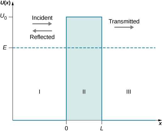
The potential in the three regions are defined by

\[\begin{equation} U(x) = \begin{cases} 0, & \mbox{when } x < 0 \\[4pt] U_0, & \mbox{when } 0 \leq x \leq L \\[4pt] 0, & \mbox{when } x > L \end{cases} \label{PIBPotential} \end{equation}\]

The potential $U(x)$ in ($\ref{PIBPotential}$) satisfy the Schrödinger equation

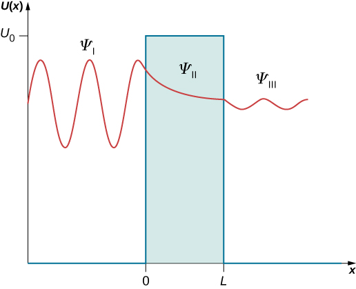
\[\begin{equation}\label{PIBSchrodinger} -\frac{\hbar^2}{2m} \frac{d^2\psi}{dx^2} + U(x)\psi = E\psi \end{equation}\]

Since the particle energy is $E$ and is less than $U_0$ in region-II therefore the solution of ($\ref{PIBSchrodinger}$) is exponentially decaying. The solution of ($\ref{PIBSchrodinger}$) in region-I and region-III are given by plane waves as particle energy is greater than the potential energy in these regions. We expect the solution to be of the form given in figure below:

We write the general solution of ($\ref{PIBSchrodinger}$) in region-I, region-II and region-III as

\[\begin{equation} \psi(x) = \begin{cases} Ae^{ikx} + Be^{-ikx}, & \mbox{when } x < 0 \\ Ce^{\lambda x} + De^{-\lambda x}, & \mbox{when } 0 \leq x \leq L \\ Fe^{ikx} + Ge^{-ikx}, & \mbox{when } x > L \end{cases} \label{PIBGeneralSolution} \end{equation}\]

where $k = \sqrt{\frac{2mE}{\hbar^2}}$ and $\lambda = \sqrt{\frac{2m(U_0-E)}{\hbar^2}}$ . The coefficient $G$ in region III is zero as there is no incident wave from right side. The continuity of wave function and its derivative at $x = 0$ and $x = L$ gives the following equations

\[\begin{equation} \begin{aligned} A + B & = C + D, \\ ik(A - B) & = \lambda(C - D), \quad \text{Derivative}\\ Ce^{\lambda L} + De^{-\lambda L} & = Fe^{ikL}, \\ \lambda(Ce^{\lambda L} - De^{-\lambda L}) & = ik Fe^{ikL} \quad \text{Derivative} \end{aligned} \label{PIBContinuity} \end{equation}\]

We have four equations ($\ref{PIBContinuity}$) and five unknowns $A$, $B$, $C$, $D$ and $F$. But the quantity of our interest is the transmission coefficient $ T $ and therefore $\frac{F}{A}$ is the quantity of interest. We therefore divide each equation by $A$ and get the ratio coefficients in terms of $A$ as

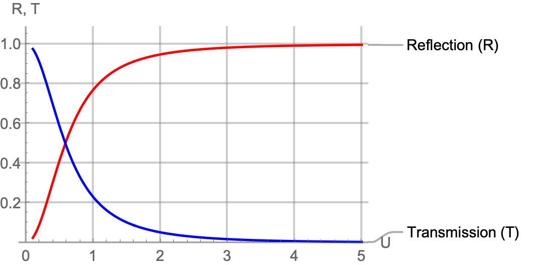
$\begin{equation} \begin{aligned} 1 + \frac{B}{A} & = \frac{C}{A} + \frac{D}{A}, \\ ik(1 - \frac{B}{A}) & = \lambda(\frac{C}{A} - \frac{D}{A}), \\ \frac{C}{A}e^{\lambda L} + \frac{D}{A}e^{-\lambda L} & = \frac{F}{A}e^{ikL}, \\ \lambda(\frac{C}{A}e^{\lambda L} - \frac{D}{A}e^{-\lambda L}) & = ik \frac{F}{A}e^{ikL} \end{aligned} \label{PIBContinuityRatio} \end{equation}$ Solving for $\frac{F}{A}$ we get $\begin{equation} \frac{F}{A} = \frac{ e^{-i k L}}{\cosh (\lambda L)+\frac{i}{2}(\frac{\lambda}{k}-\frac{k}{\lambda}) \sinh (\lambda L)} \label{PIBTransmission} \end{equation}$ The transmission coefficient $T$ is given by $\begin{equation} T=|\frac{F}{A}|^2 = \frac{ 1}{\cosh^2 (\lambda L)+\frac{1}{4}(\frac{\lambda}{k}-\frac{k}{\lambda})^2 \sinh^2 (\lambda L)} \label{PIBTransmissionCoefficient} \end{equation}$ Similarly the reflection coefficient $R$ is given by $\begin{equation} R = |\frac{B}{A}|^2 =\frac{1}{\frac{4 k^2 \lambda ^2 \text{csch}^2(\lambda L)}{\left(k^2+\lambda ^2\right)^2}+1} \label{PIBReflectionCoefficient} \end{equation}$ One can check that $T + R = 1$ as expected. The Transmission coefficient can be represented as a function of $U$ and $E$ as $\begin{equation} T = \frac{1}{1+\frac{U^2}{8 (E^2-U^2)}\left(1- \cosh \left(2 L \sqrt{\frac{2m (U-E)}{\hbar ^2}}\right)\right)}\label{PIBT} \end{equation}$ The Transmission and Reflection coefficient is plotted as a function of $U$ in the figure below keeping $\hbar^2=2m=1,\;L=1$ and $E=0.1$:

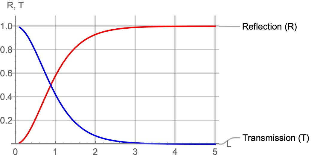
Similarly the Transmission and Reflection coefficient is plotted as a function of $L$ in the figure below keeping $\hbar^2=2m=1,\;U=2$ and $E=1$:

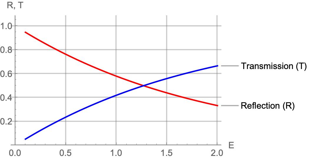
The Transmission and Reflection coefficient is plotted as a function of $E$ in the figure below keeping $\hbar^2=2m=1,\;U=2$ and $L=1$:

Observations:

The Transmission coefficient increases with an increase in $E$, while it decreases with an increase in $U$ and $L$. This behavior is consistent with the tunneling phenomena, where higher energy ($E$) increases the likelihood of transmission, and higher potential barrier ($U$) or width ($L$) suppresses it.
The wave function is exponentially decaying in region-II (inside the barrier) and takes the form of a plane wave in region-I (before the barrier) and region-III (after the barrier).
In region-I and region-III, the wave function is oscillatory and normalizable over finite spatial intervals. However, for extended or infinite domains, non-normalizable wavefunctions are encountered due to the scattering nature of the problem. Potentials of this type can give rise to quasi-bound states, characterized by resonances rather than bound energy levels.
In Quasi-Bound states, the probability density is not defined globally due to non-normalizability. Instead, the probability current is used to describe the behavior of the system. The probability current is conserved across all three regions, ensuring the continuity of physical observables.
The conservation of probability current leads to the derivation of reflection and transmission coefficients, providing quantitative measures of how the wave interacts with the potential barrier.

Few Quasi-Bound Potentials that exhibit Tunneling

Nuclear Potential Model: Attractive and Repulsive Interactions

The nuclear potential is modeled to represent the interactions between nucleons (protons and neutrons) within an atomic nucleus. The attractive nuclear force between nucleons is depicted by a negative potential well, which holds the nucleons together. This attractive force is short-range, meaning it becomes effective only within the confines of the nucleus. Outside the nucleus, the electrostatic repulsion between protons (due to their positive charge) dominates, represented by a $\frac{1}{r}$ potential, which increases as the distance between particles increases. This electrostatic repulsion counteracts the attractive nuclear force at larger distances, ensuring that the nucleons are confined to the nucleus but still experience repulsion as they move further apart.

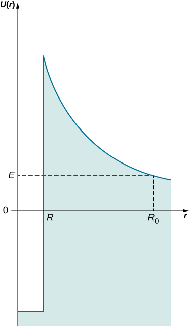
Tunneling phenomena: An alpha particle can be emitted or absorbed through quantum tunneling. When the nucleus has enough energy to overcome the potential barrier created by the electrostatic repulsion, the alpha particle (comprising two protons and two neutrons) can escape the nucleus. This process, known as alpha decay, is facilitated by tunneling through the potential barrier, despite the particle’s energy being lower than the barrier height. Conversely, an alpha particle can also be absorbed by the nucleus if the incoming particle’s energy and the potential conditions align, leading to an increase in the nucleus’s energy state.

Resonant-Tunneling Diode and Quantum Dot Mechanism:

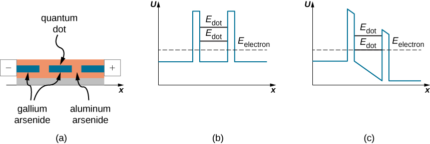
Resonant-Tunneling Diode: (a) A gallium arsenide quantum dot embedded in aluminum arsenide. (b) A potential well with two barriers and no voltage bias, where electron energies in aluminum arsenide do not align with the quantum dot's energy levels, preventing tunneling. (c) The potential well with an applied voltage bias, aligning the electron energies in the dot and aluminum arsenide, enabling tunneling through the dot.

In resonant tunneling devices, quantum dots act as potential wells with quantized energy levels for electrons. These dots are embedded in semiconductor materials, where potential barriers exist at the dot boundaries. Electrons outside the dot cannot tunnel through unless their energy matches the quantized energy level inside the dot. This alignment occurs when an external voltage bias lowers one of the barriers, allowing tunneling to occur. As the bias is increased further, alignment is lost and tunneling stops. When the bias is adjusted to match the next energy level, tunneling resumes. This energy-dependent tunneling is the key mechanism in resonant-tunneling diodes, enabling high-speed switching in nano-electronic devices.

Scattering Problems:

In quantum mechanics, the scattering nature of a problem involves the interaction of a particle (or wave) with a potential barrier, resulting in partial reflection and transmission. Unlike bound state problems, where particles are confined, scattering problems describe particles free to move before and after encountering the potential. These problems feature wave functions that extend to infinity and are not square-integrable, requiring flux conservation for analysis.

Key characteristics of scattering problems include:

Unbounded domains: The wave functions extend infinitely in space and cannot be normalized to unity, unlike bound states.
Superposition of waves: The wave function is a combination of an incident wave (approaching the potential), a reflected wave (bouncing back), and a transmitted wave (continuing beyond the potential).
Continuity across boundaries: The wave function and its derivative remain smooth and continuous at the boundaries of the potential, ensuring accurate computation of reflection and transmission probabilities.
Oscillatory, non-normalizable solutions: The wave functions oscillate and cannot be normalized, so flux conservation through probability current is used to describe the system’s behavior.

Rosen-Morse Potential

The Rosen-Morse potential is a model potential in quantum mechanics given by:

\[V(x) = -V_0 \, \text{sech}^2(x) + \lambda \, \tanh(x),\]

where $ V_0 $ represents the depth of the potential, and $ \lambda $ introduces an asymmetry in the potential. This potential is widely used because it is exactly solvable and provides insights into both bound states and scattering states.

Bound States

For specific energy levels less than the asymptotic value of the potential, $ E < 0 $, the particle remains localized within the potential well.
The wave functions for bound states are normalizable and decay exponentially outside the well, indicating confinement.
The discrete energy spectrum of bound states depends on the parameters $ V_0 $ and $ \lambda $, reflecting the depth and asymmetry of the well.

As an example consider the symmetric Rosen-Morse potential with $ V_0 = 12 $ and $ \lambda = 0 $. The potential has the following shape as shown in figure below:

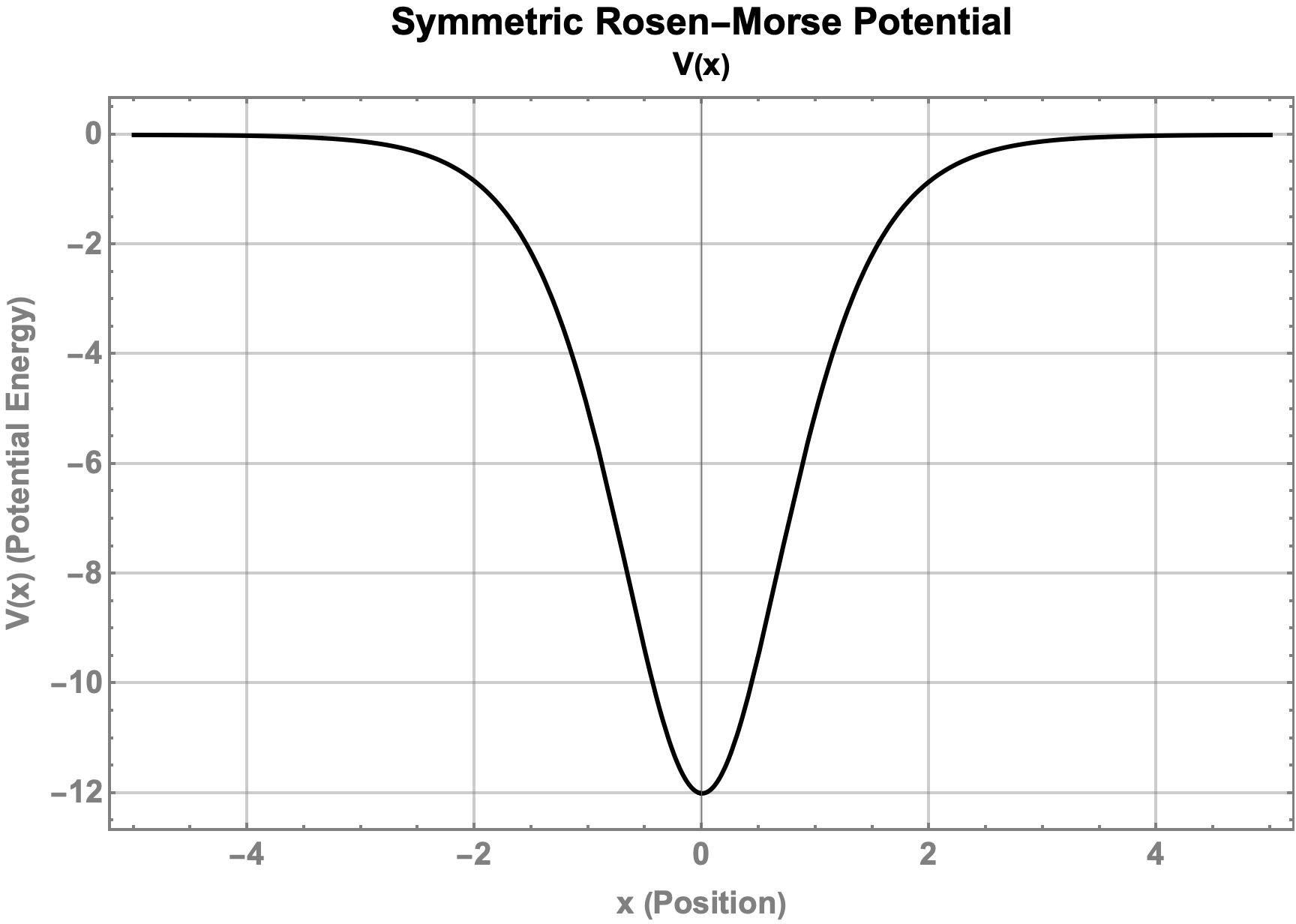
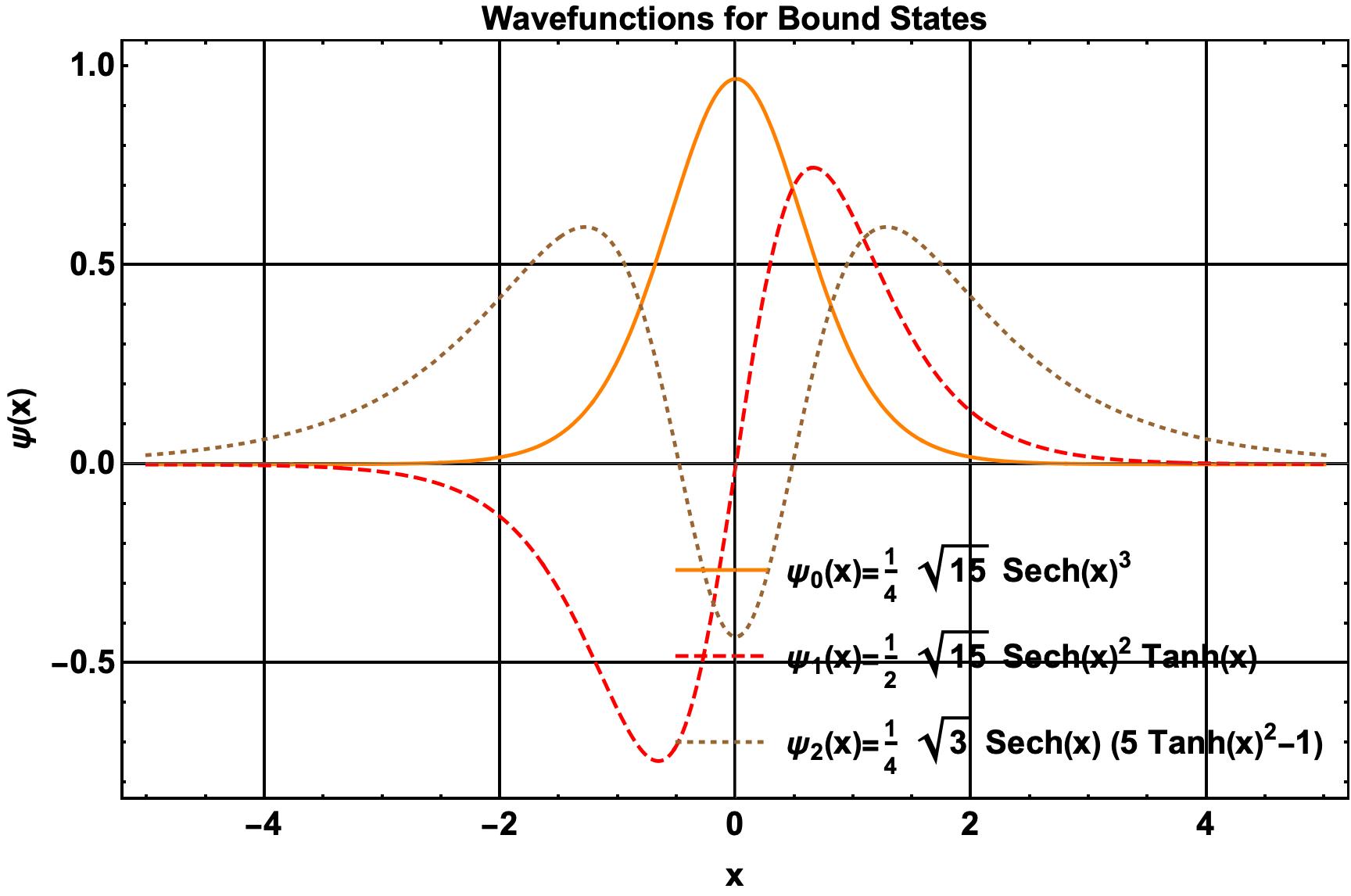
The energy and bound state wave functions are $\begin{equation} \begin{aligned} E_0 & = -9, & \psi_0(x) & = \sqrt{\frac{15}{16}} \, \text{sech}^3(x), \\ E_1 & = -4, & \psi_1(x) & = \sqrt{\frac{15}{4}} \, \text{sech}^2(x) \, \text{tanh}(x), \\ E_2 & = -1, & \psi_2(x) & = \sqrt{\frac{3}{16}} \, \text{sech}(x) \, \left( 5 \, \text{tanh}^2(x) - 1 \right). \end{aligned} \label{RosenMorseBound} \end{equation}$ There are only three bound states for the symmetric Rosen-Morse potential. The wave functions are normalized to unity and exhibit exponential decay outside the potential well as shown in figure below. For energy levels beyond the potential asymptote, the particle transitions to scattering states.

Scattering States

When the particle’s energy exceeds the potential asymptote, $ E > 0 $, it transitions to a scattering regime.
In scattering states, the wave function describes a free particle that interacts with the potential but is not confined.
The wave function exhibits oscillatory behavior, representing incident, reflected, and transmitted waves.
The reflection and transmission coefficients depend on $ V_0 $, $ \lambda $, and the particle’s energy, showing how the potential influences scattering behavior.

Physical Significance

The Rosen-Morse potential is significant because it demonstrates the coexistence of bound and scattering states in a single potential framework. Bound states represent localized solutions, while scattering states describe delocalized solutions, highlighting the dual nature of quantum systems depending on the energy of the particle relative to the potential landscape.