1. Introduction

This project simulates the motion of an N-body mass-spring system where multiple masses are connected via springs and constrained to move horizontally on a frictionless surface. The simulation involves both numerical solutions to the equations of motion and a graphical animation using PyGame.

The motivation for this study arises from its relevance in:

• Understanding lattice vibrations in solid state physics,
• Modeling mechanical systems in classical dynamics,
• Exploring numerical ODE solvers and interactive simulation frameworks.

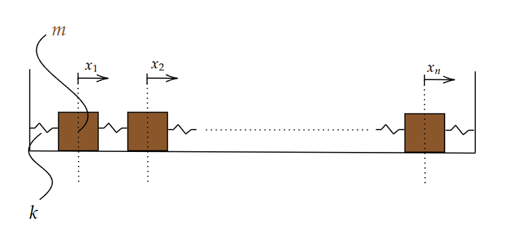
2. System Description

• The system consists of n identical masses.
• Each mass is connected to its neighbors using linear springs.
• The surface is perfectly frictionless, so there is no damping.
• All masses are initially at rest, and motion is initiated only through initial displacements.

The structure is linear, and fixed boundary conditions are typically assumed at the ends, although this can be generalized.

3. Assumptions

• All masses \(m\) are identical.
• All springs have the same spring constant \(k\).
• Motion is constrained to 1D horizontal motion.
• The springs obey Hooke’s law (linear restoring force).
• The system starts from rest, i.e., initial velocities are zero.

4. Mathematical Modeling

For each mass \(i\) (\(1 \leq i \leq n\)), Newton’s second law gives:

\[m \frac{d^2 x_i}{dt^2} = -k(x_i - x_{i-1}) + k(x_{i+1} - x_i)\]

Rewriting:

\[\frac{d^2 x_i}{dt^2} = \frac{k}{m} (x_{i+1} - 2x_i + x_{i-1})\]

This is a system of coupled second-order ODEs, forming a discrete wave equation. Special cases:

• For \(i = 1\): left boundary (may be fixed or free),
• For \(i = n\): right boundary.

This system can be written in matrix form:

\[\mathbf{M} \ddot{\mathbf{x}} = -\mathbf{Kx}\]

where:

• \(\mathbf{x}\) is the position vector,
• \(\mathbf{M} = m \mathbf{I}\) is the mass matrix,
• \(\mathbf{K}\) is the stiffness matrix (tridiagonal).

5. Numerical Integration

To solve the equations of motion, we apply numerical methods such as:

• Euler’s method (simplest, not very accurate),
• Verlet integration (commonly used in physics),
• SciPy’s solve_ivp with RK45 or RK23 solvers.

The user inputs initial displacements for each mass, and the system automatically generates:

• The stiffness matrix based on n,
• Initial state vectors for position and velocity,
• Solution over a specified time interval.

6. Visualization and Simulation

6.1 Matplotlib Plot

The displacement of each mass over time is first visualized using matplotlib.pyplot, typically as:

• Line plots of \(x_i(t)\) vs time,
• Optional animation using FuncAnimation.

6.2 PyGame Animation

Once the numerical solution is complete, a PyGame-based animation shows the physical behavior:

• Masses oscillate horizontally,
• Springs are drawn as dynamic lines,
• The background (floor.jpg) is customizable.

This animation helps build intuitive understanding of oscillatory motion and energy exchange in coupled systems.

7. User Interaction

• The user provides a list of initial positions (e.g., [1.0, -1.5, 0.3]) to define the system.
• Each input corresponds to a new mass.
• The user can customize:
  • Background image,
  • Mass and spring appearance,
  • Simulation speed.

8. Applications and Extensions

• Lattice vibrations: Ideal for simulating 1D phonons.
• Signal propagation: Observing how disturbances travel through coupled media.
• Modes of vibration: Visualize normal modes and beat phenomena.
• Nonlinear springs: Can be extended by replacing Hooke’s law with nonlinear force models.

9. Files and Structure

• mass_spring_simulation.py: Main simulation script,
• floor.jpg: Background image (user replaceable),
• utils.py: Helper functions for drawing and integration,
• initial_conditions.txt: Optional file for storing default states.