Tight-Binding Approximation
Nearly Free Electron Model and Energy Bands in One Dimension, Tight-Binding Approximation
Learning Objectives:
- Understand the basic assumptions of the nearly free electron model and how it modifies the free electron theory.
- Analyze the formation of energy bands and gaps due to weak periodic potentials.
- Learn the tight-binding approximation and how it leads to discrete energy levels forming bands.
Key Concepts / Definitions:
- Nearly Free Electron Model: A quantum mechanical model where electrons are treated as nearly free, slightly perturbed by a weak periodic potential.
- Energy Band: A range of allowed energies for an electron in a crystal due to the periodic potential.
- Tight-Binding Approximation: An approach assuming electrons are tightly bound to atoms but can hop to neighboring sites, resulting in band formation.
Nearly Free Electron Model (NFEM)
In the free electron model, electrons move in a constant potential, leading to continuous energy levels described by:
\[E = \frac{\hbar^2 k^2}{2m}\]However, in a crystal, electrons feel a periodic potential due to the lattice:
\[V(x) = V(x + a)\]where $a$ is the lattice spacing. Bloch’s theorem tells us the solutions are of the form:
\[\psi_k(x) = e^{ikx} u_k(x)\]where $u_k(x)$ has the same periodicity as the lattice.
Due to the periodic potential, energy levels are no longer continuous. Instead, band gaps open at the Brillouin zone boundaries where Bragg reflection occurs. For 1D, the Bragg condition is:
\[k = \pm \frac{n\pi}{a}, \quad n = 1, 2, 3, \ldots\]Near these points, the electron wavefunctions interfere destructively, leading to a forbidden energy gap.
This model modifies the dispersion relation near the zone boundaries, and leads to energy bands separated by gaps. The first Brillouin zone extends from $- \frac{\pi}{a}$ to $+ \frac{\pi}{a}$.
The Tight-Binding Model
The tight-binding model is a discrete approximation for understanding electron motion in solids. In this framework, space is replaced by a lattice of discrete points, corresponding to atomic positions in a crystalline solid. An electron is allowed to sit only on these discrete sites and can hop to neighboring sites due to quantum tunneling.
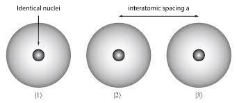
We begin by considering a one-dimensional lattice of atoms, described by $ N $ points along a line, each separated by a lattice constant $ a $. A single electron is considered, which can reside on any of these lattice sites but not in between. This assumption is central to the tight-binding approximation, which models electrons as being tightly bound to atoms with a small probability to move to neighboring sites.
Let $ \ket{n} $ denote the state where the electron is located at the $ n $-th site. These states are orthogonal:
\[< n | m > = \delta_{nm}\]The Hilbert space is $ N $-dimensional and spanned by the orthonormal set $ { |n> }_{n=1}^N $.
Hamiltonian Without Hopping
If the electron is bound to its site and never hops, the Hamiltonian $ H_0 $ is given by:
\[H_0 = E_0 \sum_{n} |n>< n|\]Each $ \ket{n}$ is an eigenstate with energy $ E_0 $. This Hamiltonian describes electrons that are completely localized and hence is trivial.
Introducing Hopping
To incorporate tunneling between sites, we modify the Hamiltonian. Quantum time evolution implies that to move an electron from one site to another, the Hamiltonian should include terms like $ |m>< n| $, which annihilates an electron at site $ n $ and creates one at site $ m $.
To keep the model local (i.e., allow only hopping to nearest neighbors), the full tight-binding Hamiltonian becomes:
\[H = E_0 \sum_{n} | n>< n| - t \sum_{n} \left( |n>< n+1| + |n+1>< n| \right)\]Here, $ t $ is the hopping parameter, determining the strength of tunneling. It must be real to ensure $ H $ is Hermitian.
We impose periodic boundary conditions by identifying $|N+1> \equiv \ket{1} $, effectively wrapping the 1D lattice into a circle. This simplifies calculations and makes the model translationally invariant.
Solving the Model
We look for energy eigenstates of $ H $. A general state is:
\[|\psi> = \sum_{m} c_m |m>\]and when operated by $<n|$ we get
\[\psi_n=<n|\psi>\]Substituting into the Schrödinger equation $ H|\psi> = E|\psi> $ and projecting onto $ < n| $, we obtain:
\[E_0 \psi_n - t (\psi_{n+1} + \psi_{n-1}) = E \psi_n\]This is a second-order difference equation, often solved by the ansatz:
\[\psi_n = e^{ikna}\]or normalized as:
\[\psi_n = \frac{1}{\sqrt{N}} e^{ikna}\]Here, $ k $ is the wavenumber, analogous to momentum. Substituting into the difference equation gives the energy dispersion relation:
\[E(k) = E_0 - 2t \cos(ka)\]This relation defines a band of allowed energies:
\[E(k) \in [E_0 - 2t, E_0 + 2t]\]The total width of the band is $ 4t $, referred to as the bandwidth.
Brillouin Zone and Quantization
Due to periodicity, $ k $ is defined modulo $ 2\pi/a $, and lies within the Brillouin zone:
\[k \in \left( -\frac{\pi}{a}, \frac{\pi}{a} \right]\]Periodicity also requires:
\[\psi_{n+N} = \psi_n \Rightarrow e^{ikNa} = 1 \Rightarrow k = \frac{2\pi}{Na} \cdot m,\quad m \in \mathbb{Z}\]Thus, $ k $ is quantized in units of $ 2\pi/(Na) $, giving exactly $ N $ distinct values, consistent with the Hilbert space dimension.
Physical Interpretation
-
Delocalization: Even for arbitrarily small $ t $, the eigenstates become completely delocalized across the entire lattice. The presence of any hopping term destroys the localization of the $ H_0 $ eigenstates.
-
Degeneracy Lifting: The degeneracy of $ H_0 $ is lifted. The spectrum now forms a band with energy varying with $ k $.
-
Effective Mass: For small $ k \ll \pi/a $, we can expand the cosine:
\[\cos(ka) \approx 1 - \frac{(ka)^2}{2} \Rightarrow E(k) \approx (E_0 - 2t) + ta^2 k^2\]This is similar to a free particle dispersion:
\[E_{\text{free}} = \frac{\hbar^2 k^2}{2m}\]Hence, the electron behaves as if it moves in a continuum with effective mass:
\[m^* = \frac{\hbar^2}{2ta^2}\] -
Position-Momentum Reciprocity:
- Making space finite or periodic quantizes momentum (as in the particle-in-a-box model).
- Making space discrete (as in tight-binding) makes momentum periodic, confined within the Brillouin zone.
- This reflects a fundamental duality: discreteness in one domain implies compactness in the other, a manifestation of Fourier duality.
The tight-binding model, despite its simplicity, captures key features of electron dynamics in solids: band formation, delocalization, and the emergence of effective mass. It serves as a starting point for more complex models including multi-band structures, disorder, and interactions.
Solved Examples:
-
Example 1:
Problem: For a 1D crystal with lattice constant $a = 2$ Å and hopping integral $t = 2$ eV, find the energy at $k = 0$ and $k = \frac{\pi}{a}$ in the tight-binding approximation.
Solution:
Given:
\(E(k) = E_0 - 2t \cos(ka)\)
At $k = 0$:
\(E(0) = E_0 - 2t = E_0 - 4 \, \text{eV}\)
At $k = \frac{\pi}{a}$:
\(E\left(\frac{\pi}{a}\right) = E_0 - 2t \cos(\pi) = E_0 + 2t = E_0 + 4 \, \text{eV}\) -
Example 2:
Problem: Estimate the width of the first band gap in a nearly free electron model for a weak periodic potential $V(x) = V_0 \cos\left(\frac{2\pi x}{a}\right)$.
Solution:
Band gap opens at $k = \pm \frac{\pi}{a}$. The energy gap is approximately:
\(\Delta E \approx |V_G| = \left| \frac{1}{a} \int_0^a V(x) e^{-i \frac{2\pi x}{a}} dx \right| = |V_0|\)
Thus, the band gap is approximately equal to the Fourier component of the potential at the reciprocal lattice vector $G = \frac{2\pi}{a}$.
Important Points / Summary:
- Nearly free electron model explains the origin of band gaps due to Bragg reflection in periodic potentials.
- The formation of allowed and forbidden energy regions leads to conduction and valence bands.
- Tight-binding model is useful for materials with localized electrons and predicts cosine-shaped energy bands.
Practice Questions:
- Short Answer:
- What is the physical significance of a band gap in solids?
- Explain why energy gaps appear at the Brillouin zone boundaries in the nearly free electron model.
- Numerical:
- Calculate the bandwidth for a tight-binding band with $t = 1.5$ eV.
- If the periodic potential has strength $V_0 = 0.8$ eV, estimate the band gap at $k = \pm \frac{\pi}{a}$.
- MCQs:
- In the tight-binding model, the energy dispersion relation is:
- (A) $E(k) = \frac{\hbar^2 k^2}{2m}$
- (B) $E(k) = E_0 - 2t \cos(ka)$
- (C) $E(k) = E_0 + tk$
- (D) $E(k) = E_0 + t \sin(ka)$
Answer: (B)
- The first Brillouin zone for a 1D crystal with lattice spacing $a$ extends from:
- (A) $0$ to $\frac{2\pi}{a}$
- (B) $-\frac{\pi}{a}$ to $\frac{\pi}{a}$
- (C) $-\frac{2\pi}{a}$ to $\frac{2\pi}{a}$
- (D) $0$ to $\frac{\pi}{a}$
Answer: (B)
- In the tight-binding model, the energy dispersion relation is: