Classical mechanics can be read as a continuous shift from a force-first description to a structure-first description. Each stage keeps the same physical predictions but changes the language so that constraints, symmetries, and conserved quantities become simpler to express. The progression moves from forces and accelerations to variational principles, then to phase-space geometry, and finally to generators and Poisson-bracket algebra.

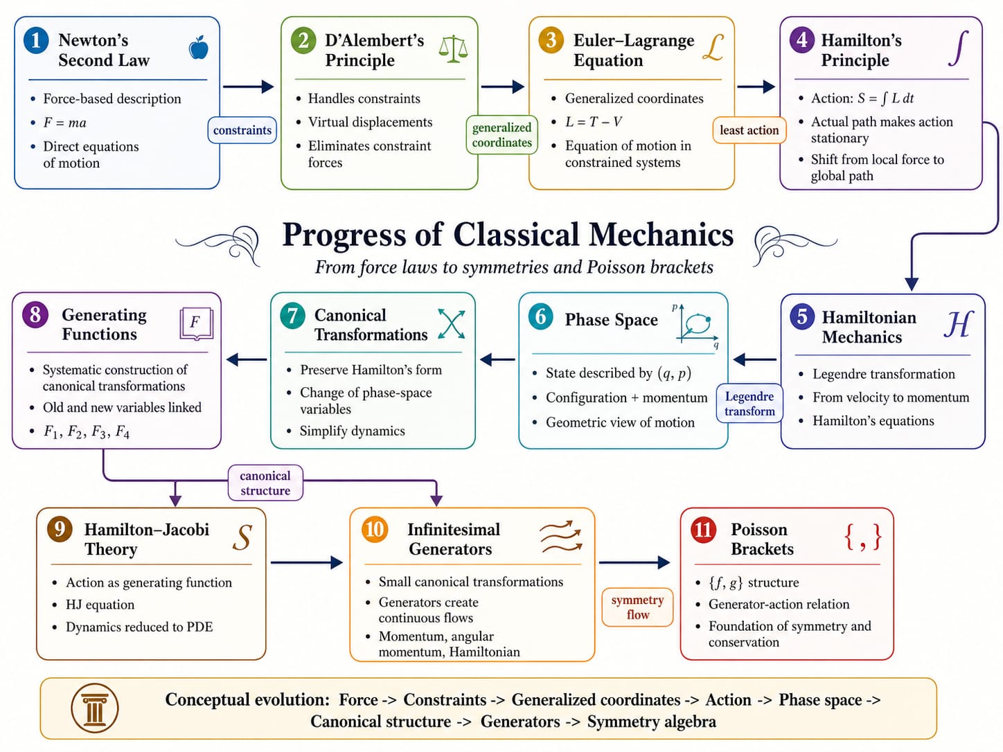
From Newton’s Law to D’Alembert and Constraints

Newton’s second law,

\[\mathbf{F}=m\mathbf{a},\]

describes motion through forces and accelerations in Cartesian coordinates. For unconstrained problems this is direct, but in constrained systems (beads on wires, pendula, rolling, rigid linkages, many-particle constraints) the difficulty is that constraint forces are often unknown and must be solved along with the motion.

D’Alembert’s principle isolates the physically effective part of the forces by using virtual displacements $\delta\mathbf{r}_i$ compatible with the constraints. Writing Newton’s law as $\mathbf{F}-m\mathbf{a}=0$ and taking virtual work gives

\[\sum_i(\mathbf{F}_i-m_i\mathbf{a}_i)\cdot \delta \mathbf{r}_i=0.\]

For ideal constraints, the constraint forces do no virtual work, so they drop out automatically. This is the first conceptual reorganization: instead of tracking all forces, one tracks only the allowed motions consistent with the constraints.

Lagrange’s Equations and Hamilton’s Principle

Generalized coordinates $q_i$ parametrize the independent degrees of freedom of the constrained system. The kinetic and potential energies become functions of $(q,\dot q,t)$, and the Lagrangian is

\[L=T-V.\]

From D’Alembert’s principle expressed in generalized coordinates, one obtains the Euler–Lagrange equations

\[\frac{d}{dt}\left(\frac{\partial L}{\partial \dot q_i}\right)-\frac{\partial L}{\partial q_i}=0.\]

Hamilton’s principle then supplies the deeper organizing idea: motion is not viewed as being pushed instant by instant, but as a path selected by a variational condition. The action is

\[S=\int_{t_1}^{t_2}L(q,\dot q,t)\,dt,\]

and the physical path satisfies

\[\delta S=0.\]

The Euler–Lagrange equations are the local differential consequence of this global statement about competing paths between fixed endpoints. This shift—from forces to stationary action—makes symmetry and conservation statements natural and prepares the transition to phase-space structure.

Hamiltonian Mechanics, Canonical Transformations, and Hamilton–Jacobi

The Legendre transformation replaces velocities by conjugate momenta:

\[p_i=\frac{\partial L}{\partial \dot q_i},\]

and defines the Hamiltonian

\[H(q,p,t)=\sum_i p_i\dot q_i-L.\]

The equations of motion become Hamilton’s equations,

\[\dot q_i=\frac{\partial H}{\partial p_i},\] \[\dot p_i=-\frac{\partial H}{\partial q_i}.\]

This is the second major shift: the state is described in phase space by $(q_i,p_i)$, and dynamics becomes a flow on that space. Once phase space is central, one asks which changes of variables preserve the form of Hamilton’s equations. This leads to canonical transformations

\[(q,p)\longrightarrow (Q,P),\]

which preserve the Hamiltonian structure. Such transformations are constructed systematically using generating functions. For a generating function $F_2(q,P,t)$, the transformation is encoded by

\[p_i=\frac{\partial F_2}{\partial q_i},\] \[Q_i=\frac{\partial F_2}{\partial P_i}.\]

Hamilton–Jacobi theory is the sharpest application of this idea: one seeks a canonical transformation generated by Hamilton’s principal function $S(q,\alpha,t)$ such that the transformed Hamiltonian becomes a constant (often taken to be zero), making the new variables constants of motion. The Hamilton–Jacobi equation is

\[H\left(q_i,\frac{\partial S}{\partial q_i},t\right)+\frac{\partial S}{\partial t}=0.\]

Thus the task of integrating the equations of motion is reorganized into solving a single first-order partial differential equation for $S$, with the action functioning as a generating function for the transformation to constants of motion.

Infinitesimal Generators and Poisson Brackets

After canonical transformations, the next structural question is whether continuous transformations can be built from infinitesimal ones. Consider an infinitesimal canonical transformation

\[q_i' = q_i+\delta q_i,\] \[p_i' = p_i+\delta p_i.\]

Such a transformation is generated by a function $G(q,p,t)$, called an infinitesimal generator, with

\[\delta q_i=\varepsilon \frac{\partial G}{\partial p_i},\] \[\delta p_i=-\varepsilon \frac{\partial G}{\partial q_i}.\]

This elevates generators to a central role: continuous symmetries and phase-space flows are produced by specific functions on phase space. Standard examples include:

• momentum generates translations in position,
• angular momentum generates rotations,
• the Hamiltonian generates time evolution,
• position generates translations in momentum.

The Poisson bracket is introduced as the compact language that measures how any function on phase space changes under a generator:

\[\{f,g\}=\sum_i\left(\frac{\partial f}{\partial q_i}\frac{\partial g}{\partial p_i} -\frac{\partial f}{\partial p_i}\frac{\partial g}{\partial q_i}\right).\]

With this structure, the infinitesimal change of any dynamical quantity $f(q,p,t)$ generated by $G$ is

\[\delta f=\varepsilon \{f,G\}.\]

Time evolution appears as the special case where the generator is $H$:

\[\frac{df}{dt}=\{f,H\}+\frac{\partial f}{\partial t}.\]

In particular, Hamilton’s equations themselves become Poisson-bracket identities,

\[\dot q_i=\{q_i,H\},\] \[\dot p_i=\{p_i,H\}.\]

At this final stage, mechanics is organized as an algebra of generators and brackets: Poisson brackets specify which functions generate which transformations, identify conserved quantities, and reveal how symmetry is encoded directly into the structure of phase space.