16 Jun 2025

First-Order Homogeneous and Non-Homogeneous Differential Equations

Homogeneous first-order equations and the integrating-factor solution of linear homogeneous and non-homogeneous equations.

bsc semester-ii mathematical-physics differential-equations first-order-equations

A first-order ordinary differential equation contains $y(x)$ and $dy/dx$, but no higher derivative. Two meanings of homogeneous occur in first-order work, so they must be kept distinct.

Homogeneous in the ratio (y/x)

An equation

\[\frac{dy}{dx}=F\!\left(\frac yx\right)\]

is homogeneous because a common scaling $(x,y)\mapsto(\lambda x,\lambda y)$ leaves $y/x$ unchanged. Put

\[v=\frac yx, \qquad y=xv(x).\]

The product rule, which must not be omitted, gives

\[\frac{dy}{dx}=v+x\frac{dv}{dx}.\]

Hence

\[v+x\frac{dv}{dx}=F(v), \qquad \frac{dv}{F(v)-v}=\frac{dx}{x}.\]

Before dividing by $F(v)-v$, check whether $F(v_{\ast})=v_{\ast}$. Each such constant value gives the straight-line solution $y=v_{\ast}x$ and may otherwise be lost. After integration, substitute $v=y/x$.

For example,

\[\frac{dy}{dx}=1+\frac yx\]

becomes $v+xv^{\prime}=1+v$, so $xv^{\prime}=1$. Therefore

\[v=\ln\lvert x\rvert+C, \qquad \boxed{y=x\bigl(\ln\lvert x\rvert+C\bigr)}.\]

Differentiating the answer gives $y^{\prime}=\ln\lvert x\rvert+C+1=1+y/x$, so the original equation is recovered.

Linear homogeneous and non-homogeneous equations

A first-order linear equation is

\[\boxed{y^{\prime}+P(x)y=Q(x)}.\]

It is linear homogeneous when $Q=0$ and non-homogeneous when $Q\ne0$. To combine the two terms on the left into one derivative, multiply by a function $\mu(x)$:

\[\mu y^{\prime}+\mu Py=\frac{d}{dx}(\mu y) =\mu y^{\prime}+\mu^{\prime} y.\]

The coefficients of $y$ agree when

\[\mu^{\prime}=P\mu, \qquad \frac{d\mu}{\mu}=P(x)dx.\]

Thus an integrating factor is

\[\boxed{\mu(x)=e^{\int P(x)dx}}.\]

The multiplied equation is $(\mu y)^{\prime}=\mu Q$. Integrating between a reference point $x_0$ and $x$ gives

\[\mu(x)y(x)-\mu(x_0)y(x_0) =\int_{x_0}^{x}\mu(s)Q(s)\,ds.\]

Equivalently,

\[\boxed{ y(x)=\frac{1}{\mu(x)} \left[C+\int^x\mu(s)Q(s)\,ds\right]}.\]

For $Q=0$, this reduces to $y_h=C/\mu$. For $Q\ne0$, the answer is $y=y_h+y_p$.

Example

Solve

\[y^{\prime}+2y=e^{-x}.\]

Here $P=2$, so $\mu=e^{2x}$. Then

\[e^{2x}y^{\prime}+2e^{2x}y=(e^{2x}y)^{\prime}=e^x.\]

Therefore

\[e^{2x}y=e^x+C, \qquad \boxed{y=e^{-x}+Ce^{-2x}}.\]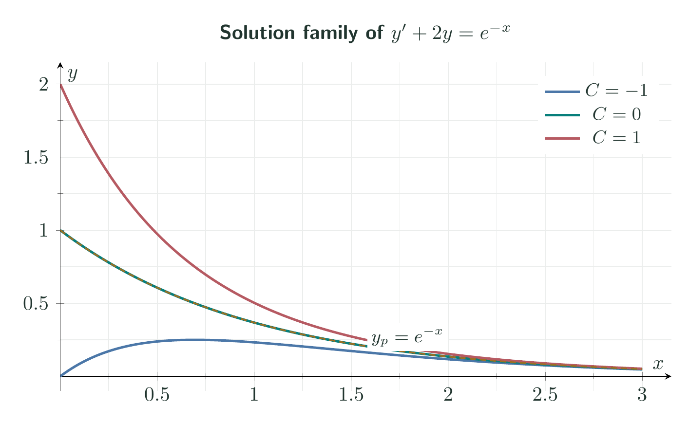

Every curve satisfies \(y^{\prime}+2y=e^{-x}\). The \(Ce^{-2x}\) part is the homogeneous freedom, while \(e^{-x}\) is one particular solution.

Substitution gives

\[y^{\prime}+2y=(-e^{-x}-2Ce^{-2x}) +2(e^{-x}+Ce^{-2x})=e^{-x}.\]

The substitutions in this post are checked in the Unit II Maxima worksheet; every reported residual is zero.

Solved Problems

1. A ratio-homogeneous initial-value problem

Solve

\[\frac{dy}{dx}=\left(\frac yx\right)^2, \qquad y(1)=2, \qquad x>0.\]

Put $y=xv$. Then $y^{\prime}=v+xv^{\prime}$ and

\[v+x\frac{dv}{dx}=v^2, \qquad \frac{dv}{v(v-1)}=\frac{dx}{x}.\]

The divided factors show that $v=0$ and $v=1$ must first be checked; they give $y=0$ and $y=x$, neither of which satisfies the initial value. For the remaining solutions,

\[\int\left(-\frac1v+\frac1{v-1}\right)dv =\int\frac{dx}{x},\]

so

\[\ln\left\lvert\frac{v-1}{v}\right\rvert =\ln x+C, \qquad \frac{v-1}{v}=Kx.\]

Thus $v=1/(1-Kx)$ and $y=x/(1-Kx)$. Since $v(1)=2$, $K=1/2$, giving

\[\boxed{y=\frac{2x}{2-x}}, \qquad 0<x<2.\]

Indeed, $y^{\prime}=4/(2-x)^2=(y/x)^2$ and $y(1)=2$. The interval stops at $x=2$, where this branch becomes singular.

2. A linear equation with a variable coefficient

Solve

\[y^{\prime}+\frac1x y=x^2, \qquad y(1)=1, \qquad x>0.\]

Here

\[\mu(x)=\exp\!\int\frac{dx}{x}=x.\]

Multiplication by $x$ gives

\[xy^{\prime}+y=(xy)^{\prime}=x^3.\]

Integrating and applying the initial condition,

\[xy=\frac{x^4}{4}+C, \qquad 1=\frac14+C, \qquad C=\frac34.\]

Therefore

\[\boxed{y=\frac{x^4+3}{4x}}.\]

Substitution gives $y^{\prime}+y/x=x^2$ exactly. With dimensionless $x$ and $y$, every term is dimensionless per unit $x$, as required.

Descriptive Questions

1. Explain why “homogeneous” has two different meanings for first-order differential equations, and state a test for each meaning.
2. Derive the substitution $y=xv$ for an equation $y^{\prime}=F(y/x)$ and explain how straight-line solutions can be lost during separation.
3. Derive the integrating factor for $y^{\prime}+P(x)y=Q(x)$ directly from the product rule.
4. Explain how an initial condition fixes the homogeneous freedom in the integrating-factor solution.

Numerical Problems

1. For $y^{\prime}=2(y/x)-(y/x)^2$, find all constant-ratio solution slopes. Final answer: $v=0,1$; hence $y=0$ and $y=x$.
2. A concentration $q(t)$ obeys $q^{\prime}+0.4q=6$, where $t$ is in seconds, $q$ is in $\mathrm{mg\,L^{-1}}$, and $q(0)=2\,\mathrm{mg\,L^{-1}}$. Find $q(5\,\mathrm{s})$. Final answer: $q=15-13e^{-0.4t}$; $q(5)=13.2406\,\mathrm{mg\,L^{-1}}$.
3. Solve $y^{\prime}+(2/x)y=x^2$, $y(1)=0$, and evaluate $y(2)$. Final answer: $y=(x^5-1)/(5x^2)$; $y(2)=31/20=1.55$.
4. A homogeneous relaxation satisfies $y^{\prime}+ky=0$ and $y(4\,\mathrm{s})=y(0)/8$. Find $k$ and the half-life. Final answer: $k=(\ln8)/4=0.51986\,\mathrm{s^{-1}}$; $t_{1/2}=4/3=1.3333\,\mathrm{s}$.

The problem solutions and numerical values are verified in the Unit II problem-check worksheet.

References

1. Homogeneous differential equation — Wikipedia
2. William E. Boyce, Richard C. DiPrima, and Douglas B. Meade, Elementary Differential Equations and Boundary Value Problems, 11th ed., chapter “First-Order Differential Equations,” Wiley.
3. Dennis G. Zill, A First Course in Differential Equations with Modeling Applications, 11th ed., chapter “First-Order Differential Equations,” Cengage.
4. Mary L. Boas, Mathematical Methods in the Physical Sciences, 3rd ed., Chapter 8, “Ordinary Differential Equations,” Wiley.