24 May 2025

Scalar and Vector Fields, Directional Derivatives, and the Gradient

Fields, directional and normal derivatives, and the geometrical meaning of the gradient.

bsc semester-ii mathematical-physics vector-calculus gradient

A field assigns a physical quantity to every point. A scalar field assigns one number,

\[\phi:\mathbb R^3\to\mathbb R, \qquad (x,y,z)\mapsto\phi(x,y,z),\]

whereas a vector field assigns a vector,

\[\mathbf A=A_x\hat{\mathbf x}+A_y\hat{\mathbf y}+A_z\hat{\mathbf z}.\]

The dimensions belong to the field: if $T$ is temperature, then $[T]={\rm K}$ and $[\partial T/\partial x]={\rm K\,m^{-1}}$.

Change of a scalar field

For $d\mathbf r=dx\,\hat{\mathbf x}+dy\,\hat{\mathbf y}+dz\,\hat{\mathbf z}$, the first-order Taylor expansion is

\[d\phi=\frac{\partial\phi}{\partial x}dx +\frac{\partial\phi}{\partial y}dy +\frac{\partial\phi}{\partial z}dz.\]

Define

\[\nabla=\hat{\mathbf x}\partial_x+\hat{\mathbf y}\partial_y+\hat{\mathbf z}\partial_z, \qquad \nabla\phi=\phi_x\hat{\mathbf x}+\phi_y\hat{\mathbf y}+\phi_z\hat{\mathbf z}.\]

Then

\[\boxed{d\phi=\nabla\phi\cdot d\mathbf r}.\]

Because $d\phi$ is a scalar, $\nabla\phi$ transforms as a vector under rotations of Cartesian axes.

Directional derivative

Move from $\mathbf r_0$ along a unit vector $\hat{\mathbf n}$:

\[\mathbf r(s)=\mathbf r_0+s\hat{\mathbf n}, \qquad \frac{d\mathbf r}{ds}=\hat{\mathbf n}.\]

The chain rule gives

\[\begin{aligned} \frac{d\phi}{ds} &=\phi_x\frac{dx}{ds}+\phi_y\frac{dy}{ds}+\phi_z\frac{dz}{ds}\\ &=\nabla\phi\cdot\hat{\mathbf n}. \end{aligned}\]

Thus

\[\boxed{D_{\hat{\mathbf n}}\phi=\hat{\mathbf n}\cdot\nabla\phi}.\]

If $\alpha$ is the angle between $\hat{\mathbf n}$ and $\nabla\phi$,

\[D_{\hat{\mathbf n}}\phi=\lvert\nabla\phi\rvert\cos\alpha.\]

The maximum value $\lvert\nabla\phi\rvert$ occurs along $\nabla\phi$; the minimum $-\lvert\nabla\phi\rvert$ occurs in the opposite direction.

Geometrical interpretation and normal derivative

On a level surface $\phi(x,y,z)=C$, a tangent displacement $d\mathbf r_{\parallel}$ leaves $\phi$ unchanged. Therefore

\[0=d\phi=\nabla\phi\cdot d\mathbf r_{\parallel}.\]

Hence $\nabla\phi$ is normal to the level surface wherever $\nabla\phi\ne\mathbf0$. Choose the unit normal in the direction of increasing $\phi$,

\[\hat{\mathbf n}=\frac{\nabla\phi}{\lvert\nabla\phi\rvert},\]

the normal derivative is

\[\boxed{\frac{\partial\phi}{\partial n} =\hat{\mathbf n}\cdot\nabla\phi=\lvert\nabla\phi\rvert}.\]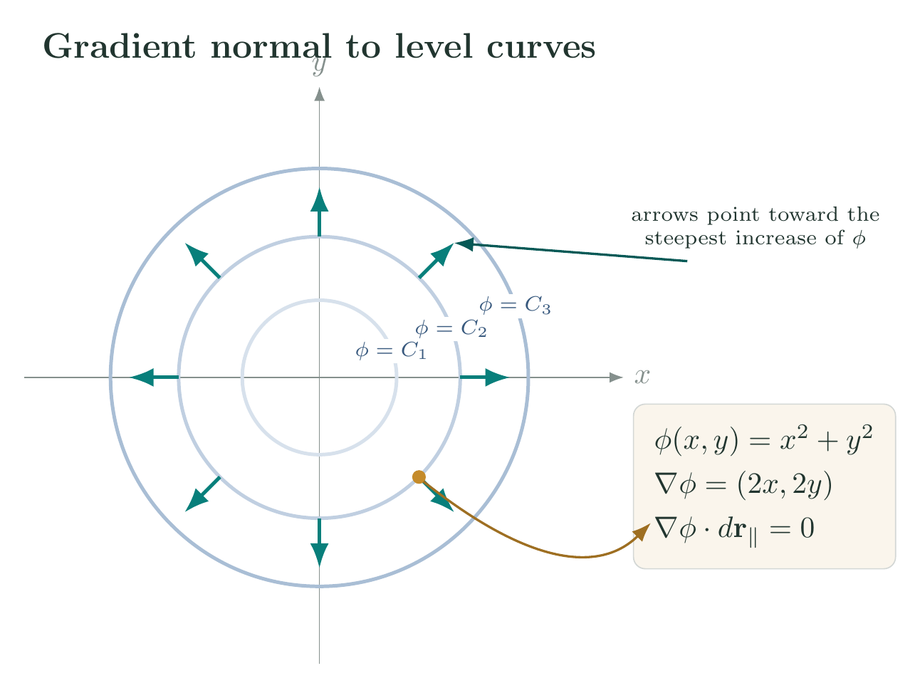

For \(\phi=x^2+y^2\), the level curves are circles and \(\nabla\phi=(2x,2y)\) is radial. The plotted curves and arrows come directly from these equations.

For $\phi=x^2+y^2+3z$,

\[\nabla\phi=2x\hat{\mathbf x}+2y\hat{\mathbf y}+3\hat{\mathbf z}.\]

At $(1,-1,0)$, along $\hat{\mathbf n}=(2,1,2)/3$,

\[D_{\hat{\mathbf n}}\phi=(2,-2,3)\cdot\frac{(2,1,2)}3 =\frac{4-2+6}{3}=\frac83.\]

If the opposite orientation is chosen, the normal derivative is $-\lvert\nabla\phi\rvert$. The units $[\nabla\phi]=[\phi]/{\rm length}$ confirm that the gradient is a spatial rate of change.