28 Jul 2025

AC Circuits, Bridges, and the Transformer

Complex impedance, series and parallel LCR resonance, power, quality factor, bandwidth, AC and resistance bridges, transformer models, vector diagram, and losses.

electricity-and-magnetism ac-circuits lcr-resonance bridges transformer

Represent a sinusoid by the real part of a complex phasor:

\[v(t)=\Re\!\left(\sqrt2\,V e^{j\omega t}\right), \qquad i(t)=\Re\!\left(\sqrt2\,I e^{j\omega t}\right),\]

where $V$ and $I$ are rms phasors and $j^2=-1$. Differentiation becomes multiplication by $j\omega$. The element impedances are

\[\boxed{Z_R=R}, \qquad \boxed{Z_L=j\omega L}, \qquad \boxed{Z_C=\frac{1}{j\omega C}=-\frac{j}{\omega C}}.\]

Their reactances are $X_L=\omega L$ and $X_C=-1/(\omega C)$. Kirchhoff’s laws retain their algebraic form for phasors:

\[\boxed{\sum_{\text{node}} I=0}, \qquad \boxed{\sum_{\text{loop}} V=0}.\]

They apply when all sources have the same angular frequency and the circuit has reached sinusoidal steady state.

Series LCR circuit

Kirchhoff’s loop law gives

\[V=IR+Ij\omega L+\frac{I}{j\omega C}.\]

Therefore

\[\boxed{Z_s=R+j\left(\omega L-\frac{1}{\omega C}\right)}\]

and

\[\lvert Z_s\rvert=\sqrt{R^2+\left(\omega L-\frac{1}{\omega C}\right)^2}.\]

The rms current and phase angle are

\[\boxed{ I=\frac{V} {\sqrt{R^2+\left(\omega L-\dfrac{1}{\omega C}\right)^2}}},\] \[\boxed{\tan\phi =\frac{\omega L-\dfrac{1}{\omega C}}{R}},\]

where the applied voltage leads the current by $\phi$. The circuit is capacitive below resonance and inductive above resonance.

Resonance

At resonance the net reactance vanishes:

\[\omega_0L-\frac{1}{\omega_0C}=0.\]

Thus

\[\boxed{\omega_0=\frac{1}{\sqrt{LC}}}, \qquad \boxed{f_0=\frac{1}{2\pi\sqrt{LC}}}.\]

At $\omega_0$, $Z_s=R$, the current is maximum, and $V_L$ and $V_C$ are equal in magnitude and opposite in phase.

Average power

Let

\[v=\sqrt2V\cos\omega t, \qquad i=\sqrt2I\cos(\omega t-\phi).\]

Using $2\cos A\cos B=\cos(A-B)+\cos(A+B)$,

\[p(t)=VI\left[\cos\phi+\cos(2\omega t-\phi)\right].\]

The second term averages to zero over a cycle, so

\[\boxed{P_{\mathrm{av}}=VI\cos\phi}.\]

Only the resistor dissipates average power:

\[\boxed{P_{\mathrm{av}}=I^2R=\frac{V^2R}{\lvert Z_s\rvert^2}}.\]

The factor $\cos\phi=R/\lvert Z_s\rvert$ is the power factor.

Half-power frequencies, bandwidth, and quality factor

At resonance $I_0=V/R$. At either half-power frequency, the current is $I_0/\sqrt2$, so

\[R^2+\left(\omega L-\frac{1}{\omega C}\right)^2=2R^2.\]

Hence

\[\left\lvert\omega L-\frac{1}{\omega C}\right\rvert=R.\]

For the lower frequency,

\[L\omega_1^2+R\omega_1-\frac1C=0,\]

which gives the positive root

\[\omega_1=\frac{-R+\sqrt{R^2+4L/C}}{2L}.\]

For the upper frequency,

\[L\omega_2^2-R\omega_2-\frac1C=0,\]

so

\[\omega_2=\frac{R+\sqrt{R^2+4L/C}}{2L}.\]

Subtracting and multiplying the roots gives

\[\boxed{\Delta\omega=\omega_2-\omega_1=\frac{R}{L}}, \qquad \boxed{\omega_1\omega_2=\omega_0^2}.\]

The series quality factor is

\[\boxed{ Q_s=\frac{\omega_0}{\Delta\omega} =\frac{\omega_0L}{R} =\frac{1}{\omega_0CR}}.\]

At resonance, $Q_s=\lvert V_L\rvert/V=\lvert V_C\rvert/V$.

Parallel LCR circuit

For ideal $R$, $L$, and $C$ branches in parallel,

\[I=V\left(\frac1R+\frac{1}{j\omega L}+j\omega C\right).\]

Thus the admittance is

\[\boxed{ Y_p=\frac1R+j\left(\omega C-\frac{1}{\omega L}\right)}.\]

At

\[\boxed{\omega_0=\frac1{\sqrt{LC}}},\]

the inductive and capacitive branch currents cancel. The source current is minimum and

\[\boxed{Z_p=\frac1{Y_p}=R}\]

is maximum.

For a fixed source current, the half-power points satisfy $\lvert Z_p\rvert=R/\sqrt2$, equivalently

\[\left\lvert\omega C-\frac{1}{\omega L}\right\rvert=\frac1R.\]

The two positive roots give

\[\boxed{\Delta\omega_p=\frac{1}{RC}},\]

and

\[\boxed{ Q_p=\frac{\omega_0}{\Delta\omega_p} =\omega_0RC =\frac{R}{\omega_0L}}.\]

This bandwidth definition uses a current-driven parallel network; with an ideal fixed-voltage source, the resistor power $V^2/R$ itself does not vary with frequency.

General bridge balance

Let a four-arm bridge have impedances $Z_1,Z_2$ in the left branch and $Z_3,Z_4$ in the right branch. The source is across the top and bottom nodes, and a null detector joins the two midpoints. With no detector current,

\[V_B=V\frac{Z_2}{Z_1+Z_2}, \qquad V_D=V\frac{Z_4}{Z_3+Z_4}.\]

Balance requires $V_B=V_D$:

\[\frac{Z_2}{Z_1+Z_2} =\frac{Z_4}{Z_3+Z_4}.\]

Cross-multiplication and cancellation of $Z_2Z_4$ give

\[\boxed{Z_1Z_4=Z_2Z_3}.\]

Because this is a complex equation, both magnitude and phase must balance in an AC bridge.

De-Sauty bridge

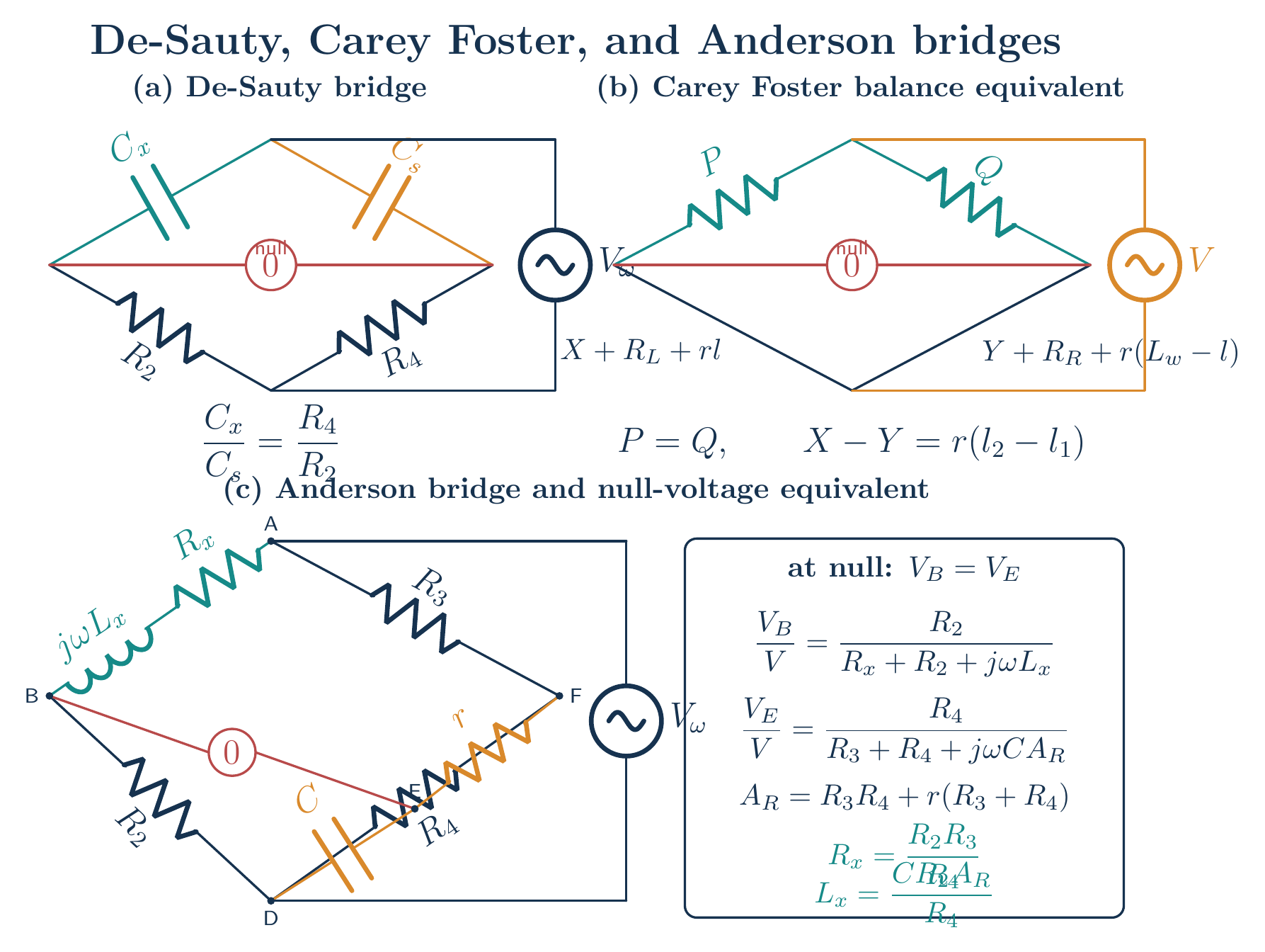
The De-Sauty bridge compares two nearly loss-free capacitances. Choose

\[Z_1=\frac{1}{j\omega C_x},\quad Z_2=R_2,\quad Z_3=\frac{1}{j\omega C_s},\quad Z_4=R_4.\]

The balance condition becomes

\[\frac{R_4}{j\omega C_x} =\frac{R_2}{j\omega C_s}.\]

Cancel $j\omega$ and cross-multiply:

\[R_4C_s=R_2C_x.\]

Therefore

\[\boxed{\frac{C_x}{C_s}=\frac{R_4}{R_2}}.\]

The result is frequency independent for ideal capacitors. Appreciable dielectric loss adds a resistive component and prevents a sharp balance with this simple bridge.

Carey Foster bridge

The Carey Foster bridge compares nearly equal resistances $X$ and $Y$. Let $r$ be the slide-wire resistance per unit length, $L_w$ its total length, $l$ a balance length measured from the left end, and $R_L,R_R$ the fixed end resistances. Choose equal ratio arms, so the two lower-arm resistances are equal at balance.

Before interchanging $X$ and $Y$,

\[X+R_L+rl_1 =Y+R_R+r(L_w-l_1).\]

After interchanging them,

\[Y+R_L+rl_2 =X+R_R+r(L_w-l_2).\]

Rearrange the first equation:

\[X-Y=R_R-R_L+rL_w-2rl_1.\]

Rearrange the second:

\[X-Y=R_L-R_R-rL_w+2rl_2.\]

Add these two expressions:

\[2(X-Y)=2r(l_2-l_1).\]

Hence

\[\boxed{X-Y=r(l_2-l_1)}.\]

The interchange cancels the unknown end corrections. The sign follows the stated left-end convention; the magnitude gives the resistance difference.

Anderson bridge

The Anderson bridge measures the series resistance $R_x$ and self-inductance $L_x$ of a real coil using a standard capacitor $C$.

Let

\[Z_x=R_x+j\omega L_x, \qquad Z_C=\frac{1}{j\omega C}.\]

The left branch is $Z_x$ in series with $R_2$. On the right, $R_3$ is in series with the parallel combination of $R_4$ and $r+Z_C$. The detector compares the junction of $Z_x,R_2$ with the junction of $r,Z_C$.

At null, no detector current flows. The left detector-node voltage is

\[\frac{V_B}{V}=\frac{R_2}{Z_x+R_2}.\]

For the right network, first form

\[Z_p=R_4\parallel(r+Z_C) =\frac{R_4(r+Z_C)}{R_4+r+Z_C}.\]

If $F$ is the junction after $R_3$, then

\[\frac{V_F}{V}=\frac{Z_p}{R_3+Z_p}, \qquad \frac{V_E}{V_F}=\frac{Z_C}{r+Z_C}.\]

Multiplying and simplifying,

\[\frac{V_E}{V} =\frac{R_4Z_C} {R_3R_4+r(R_3+R_4)+Z_C(R_3+R_4)}.\]

Divide numerator and denominator by $Z_C$, using $1/Z_C=j\omega C$:

\[\frac{V_E}{V} =\frac{R_4} {R_3+R_4+j\omega C\left[R_3R_4+r(R_3+R_4)\right]}.\]

At balance, $V_B=V_E$:

\[\frac{R_2}{R_x+R_2+j\omega L_x} = \frac{R_4} {R_3+R_4+j\omega C\left[R_3R_4+r(R_3+R_4)\right]}.\]

Equate real parts after cross-multiplication:

\[R_2(R_3+R_4)=R_4(R_x+R_2),\]

so

\[\boxed{R_x=\frac{R_2R_3}{R_4}}.\]

Equating imaginary parts gives

\[\omega R_2C\left[R_3R_4+r(R_3+R_4)\right] =\omega R_4L_x.\]

Cancel $\omega$:

\[\boxed{ L_x=\frac{CR_2}{R_4} \left[R_3R_4+r(R_3+R_4)\right]}.\]

Both ideal balance equations are independent of frequency. The equivalent voltage-divider form above also makes clear that null requires both detector voltages to have the same magnitude and phase.

Transformer

A transformer uses mutual induction between windings linked by a common alternating core flux. Let

\[\Phi(t)=\Phi_m\sin\omega t.\]

For a winding of $N$ turns,

\[e(t)=-N\frac{\mathrm d\Phi}{\mathrm dt} =-\omega N\Phi_m\cos\omega t.\]

The peak emf is $\omega N\Phi_m$, so

\[E_{\mathrm{rms}} =\frac{\omega N\Phi_m}{\sqrt2} =\sqrt2\,\pi fN\Phi_m \simeq4.44fN\Phi_m.\]

For an ideal transformer, the two windings share the same flux:

\[\boxed{\frac{V_s}{V_p} =\frac{E_s}{E_p} =\frac{N_s}{N_p}}.\]

Conservation of power and opposing ampere-turns give

\[V_pI_p=V_sI_s, \qquad N_pI_p=N_sI_s\]

in magnitude. Hence

\[\boxed{\frac{I_s}{I_p}=\frac{N_p}{N_s}}.\]

If $a=N_p/N_s$, a load $Z_L$ referred to the primary is

\[\boxed{Z_L^{\prime}=a^2Z_L}.\]

Indeed,

\[\frac{V_p}{I_p} =\frac{aV_s}{I_s/a} =a^2\frac{V_s}{I_s}.\]

Equivalent circuit of a real transformer

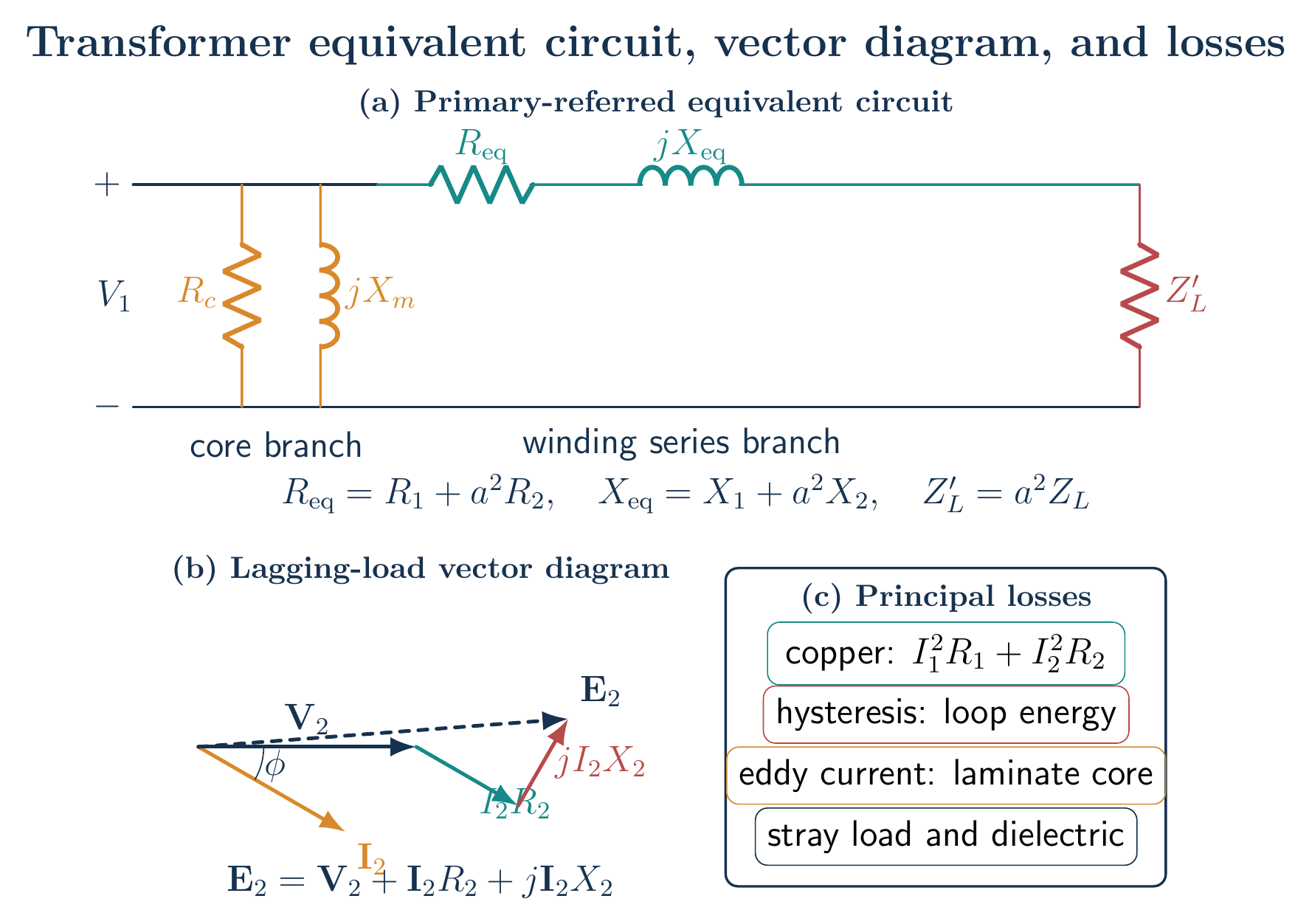
A practical winding has copper resistance $R_1,R_2$ and leakage reactance $X_1,X_2$. Core magnetization is represented by $jX_m$, while core loss is represented by $R_c$. Referred to the primary,

\[R_2^{\prime}=a^2R_2,\qquad X_2^{\prime}=a^2X_2,\qquad Z_L^{\prime}=a^2Z_L.\]

The approximate primary-referred series parameters are

\[\boxed{R_{\mathrm{eq}}=R_1+R_2^{\prime}}, \qquad \boxed{X_{\mathrm{eq}}=X_1+X_2^{\prime}}.\]

The shunt branch $R_c\parallel jX_m$ accounts for core-loss current and magnetizing current.

Vector diagram

For a lagging secondary load, take $V_2$ as reference. The current $I_2$ lags by the load angle $\phi$. The resistive drop $I_2R_2$ is in phase with $I_2$, and the leakage-reactance drop $jI_2X_2$ leads $I_2$ by $90^\circ$. Therefore

\[\boxed{\mathbf E_2 =\mathbf V_2+\mathbf I_2R_2+j\mathbf I_2X_2}.\]

With a consistent dot convention, $\mathbf E_1/\mathbf E_2=N_1/N_2$. Primary drops are added similarly to relate $\mathbf V_1$ and $\mathbf E_1$.

Transformer losses

The principal real-power losses are:

1. Copper loss

   \[\boxed{P_{\mathrm{cu}}=I_1^2R_1+I_2^2R_2}.\]

   It varies approximately as load current squared.

2. Hysteresis loss. Repeated reversal of core magnetization dissipates the $B$-$H$ loop energy every cycle. A soft, narrow-loop core reduces it.

3. Eddy-current loss. Changing flux drives circulating currents in the conducting core. Thin insulated laminations increase the transverse resistance and reduce this loss.

4. Stray load and dielectric losses. Leakage flux induces additional currents in windings and structural metal; insulation also dissipates a smaller dielectric loss.

Leakage flux mainly causes reactive voltage drop and poor regulation; associated eddy currents contribute real stray loss. At fixed supply voltage and frequency, the core loss is approximately constant, whereas copper loss changes with load. The efficiency is

\[\boxed{ \eta=\frac{P_{\mathrm{out}}} {P_{\mathrm{out}}+P_{\mathrm{cu}}+P_{\mathrm{core}}+P_{\mathrm{stray}}}}.\]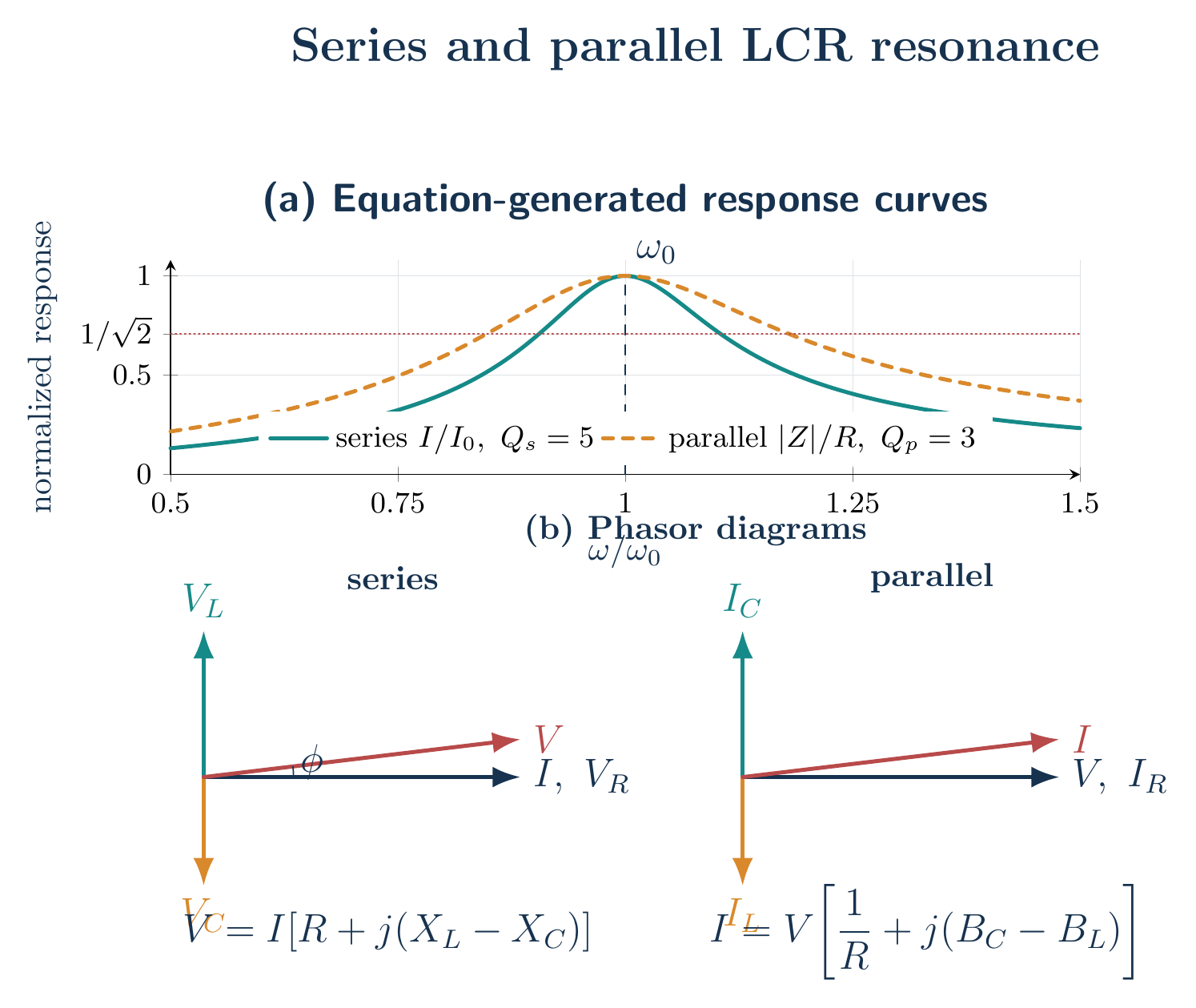

The response curves come directly from the normalized impedance equations; the phasors show reactive cancellation at resonance.

The component labels match the balance equations derived above. The Anderson panel shows both the five-arm network and the two equal detector-node voltages.

The real-transformer model separates the shunt core branch, series winding impedance, referred load, secondary vector sum, and real-power loss mechanisms.

Solved Problems

1. Design relations for a series LCR circuit

A series circuit must resonate at angular frequency $\omega_0$ with quality factor $Q$, and its capacitance $C$ is prescribed. Find $L$ and $R$.

Solution. Resonance requires

\[\omega_0=\frac{1}{\sqrt{LC}},\]

so

\[\boxed{L=\frac{1}{\omega_0^2C}}.\]

For a series circuit, $Q=\omega_0L/R$. Therefore

\[R=\frac{\omega_0L}{Q} =\boxed{\frac{1}{\omega_0CQ}}.\]

Substitution returns both the required resonance frequency and quality factor.

2. Condition for maximum transformer efficiency

Let $x$ be the fraction of full load, $P_o$ the full-load output at fixed power factor, $P_c$ the approximately constant core loss, and $P_{\mathrm{cu}}$ the full-load copper loss. Find the load for maximum efficiency.

Solution. At load fraction $x$, output is $xP_o$ and copper loss is $x^2P_{\mathrm{cu}}$. Hence

\[\eta(x)=\frac{xP_o}{xP_o+P_c+x^2P_{\mathrm{cu}}}.\]

Differentiation gives

\[\frac{\mathrm d\eta}{\mathrm dx} =\frac{P_o(P_c-x^2P_{\mathrm{cu}})} {(xP_o+P_c+x^2P_{\mathrm{cu}})^2}.\]

The stationary point is the efficiency maximum:

\[\boxed{x=\sqrt{\frac{P_c}{P_{\mathrm{cu}}}}}, \qquad \boxed{x^2P_{\mathrm{cu}}=P_c}.\]

Thus maximum efficiency occurs when variable copper loss equals constant core loss.

Descriptive Questions

1. Why can Kirchhoff’s laws be applied algebraically to phasors at a single angular frequency?
2. How do resonance and source-current behavior differ between ideal series and parallel LCR circuits?
3. Why must both magnitude and phase conditions be satisfied at the null of an AC bridge?
4. How do copper, hysteresis, eddy-current, and leakage effects appear in a real transformer?

Numerical Problems

1. Series LCR response

For $R=20.0\,\Omega$, $L=0.200\,\mathrm H$, and $C=50.0\,\mathrm{\mu F}$, find $f_0,Q$, and the half-power bandwidth $\Delta f$.

Answer: $f_0=50.3\,\mathrm{Hz}$, $Q=3.16$, and $\Delta f=15.9\,\mathrm{Hz}$.

2. Parallel LCR response

Ideal branches $R=2.00\,\mathrm{k\Omega}$, $L=0.100\,\mathrm H$, and $C=10.0\,\mathrm{\mu F}$ are in parallel. For the current-driven bandwidth definition, find $f_0,Q_p$, and $\Delta\omega_p$.

Answer: $f_0=159\,\mathrm{Hz}$, $Q_p=20.0$, and $\Delta\omega_p=50.0\,\mathrm{rad\,s^{-1}}$.

3. De-Sauty bridge

A De-Sauty bridge has $C_s=0.200\,\mathrm{\mu F}$, $R_4=600\,\Omega$, and $R_2=400\,\Omega$. Find $C_x$ at balance.

Answer: $C_x=0.300\,\mathrm{\mu F}$.

4. Carey Foster bridge

The slide wire has resistance gradient $r=0.0200\,\Omega\,\mathrm{cm^{-1}}$. Balance points before and after interchange are $l_1=35.0\,\mathrm{cm}$ and $l_2=47.0\,\mathrm{cm}$. Find $X-Y$.

Answer: $X-Y=0.240\,\Omega$.

5. Anderson bridge

An Anderson bridge has $R_2=100\,\Omega$, $R_3=200\,\Omega$, $R_4=500\,\Omega$, $r=50.0\,\Omega$, and $C=1.00\,\mathrm{\mu F}$. Find $R_x$ and $L_x$.

Answer: $R_x=40.0\,\Omega$ and $L_x=2.70\times10^{-2}\,\mathrm H$.

6. Ideal transformer

An ideal transformer has $N_p=1000$, $N_s=200$, and $V_p=230\,\mathrm V$. If the secondary current is $10.0\,\mathrm A$, find $V_s$ and $I_p$.

Answer: $V_s=46.0\,\mathrm V$ and $I_p=2.00\,\mathrm A$.

The symbolic solutions and all printed numerical answers are verified in the Unit III AC, bridges, and transformer worksheet.

References

1. RLC circuit: Wikipedia
2. Charles K. Alexander and Matthew N. O. Sadiku, Fundamentals of Electric Circuits, 7th ed., McGraw-Hill, 2021.
3. William H. Hayt, Jack E. Kemmerly, and Steven M. Durbin, Engineering Circuit Analysis, 9th ed., McGraw-Hill, 2019.
4. Stephen J. Chapman, Electric Machinery Fundamentals, 5th ed., McGraw-Hill, 2012.
5. Murray R. Spiegel, Theory and Problems of Basic Circuit Analysis, Schaum’s Outline Series, McGraw-Hill, 1974.