28 May 2025

Conductors, Capacitance, and the Method of Images

Electrostatic conductor boundary conditions, surface pressure, capacitance coefficients, and image solutions for a grounded plane and sphere.

electricity-and-magnetism conductors capacitance method-of-images

In electrostatic equilibrium, free charge in a conductor has stopped moving. Hence

\[\boxed{\mathbf E=0\quad\text{inside a conductor}}.\]

Since $\mathbf E=-\boldsymbol\nabla V$, each connected conductor is equipotential. Any excess charge resides on its surface.

Surface field, charge, and force

Let $\hat{\mathbf n}$ point from a conductor into vacuum. A thin Gaussian pillbox crossing the surface gives

\[\left(E_{n,\mathrm{out}}-E_{n,\mathrm{in}}\right)A =\frac{\sigma A}{\epsilon_0}.\]

Because $E_{n,\mathrm{in}}=0$,

\[\boxed{E_{n,\mathrm{out}}=\frac{\sigma}{\epsilon_0}}.\]

A narrow rectangular loop across the surface gives

\[\left(\mathbf E_{\mathrm{out}}-\mathbf E_{\mathrm{in}}\right) \cdot\mathrm d\mathbf l_{\parallel}=0.\]

Thus $E_{t,\mathrm{out}}=0$, and the external field is normal:

\[\boxed{\mathbf E_{\mathrm{out}} =\frac{\sigma}{\epsilon_0}\hat{\mathbf n}}.\]

The surface layer must not act on itself. The field produced by all other charge is the average of the limiting fields:

\[\mathbf E_{\mathrm{other}} =\frac{\mathbf E_{\mathrm{out}}+\mathbf E_{\mathrm{in}}}{2} =\frac{\sigma}{2\epsilon_0}\hat{\mathbf n}.\]

Therefore the outward electrostatic force per unit area is

\[\boxed{\mathbf f =\sigma\mathbf E_{\mathrm{other}} =\frac{\sigma^2}{2\epsilon_0}\hat{\mathbf n} =\frac{\epsilon_0E_{\mathrm{out}}^2}{2}\hat{\mathbf n}}.\]

The magnitude $p_e=\epsilon_0E^2/2$ is the electrostatic pressure.

Capacitance of a system of conductors

Choose infinity or an enclosing conductor as the zero of potential. Linearity of Laplace’s equation makes the conductor charges linear functions of the conductor potentials:

\[\boxed{Q_i=\sum_{j=1}^{N}C_{ij}V_j}.\]

The coefficients depend only on geometry and permittivity. Electrostatic reciprocity gives

\[C_{ij}=C_{ji},\qquad C_{ii}>0,\qquad C_{ij}\le0\quad(i\ne j).\]

Build the charges quasistatically from zero. Because $V_i$ is linear in all charges, the work is

\[W=\int_0^1\sum_i(\lambda V_i)\,Q_i\,\mathrm d\lambda =\frac12\sum_iQ_iV_i.\]

Using $Q_i=\sum_jC_{ij}V_j$,

\[\boxed{W=\frac12\sum_{i,j}C_{ij}V_iV_j}.\]

For two conductors carrying $+Q$ and $-Q$, with potential difference $\Delta V$,

\[\boxed{C=\frac{Q}{\Delta V}}, \qquad \boxed{W=\frac{Q^2}{2C}=\frac12C(\Delta V)^2}.\]

Capacitance is measured in farads.

Image charge for a grounded infinite plane

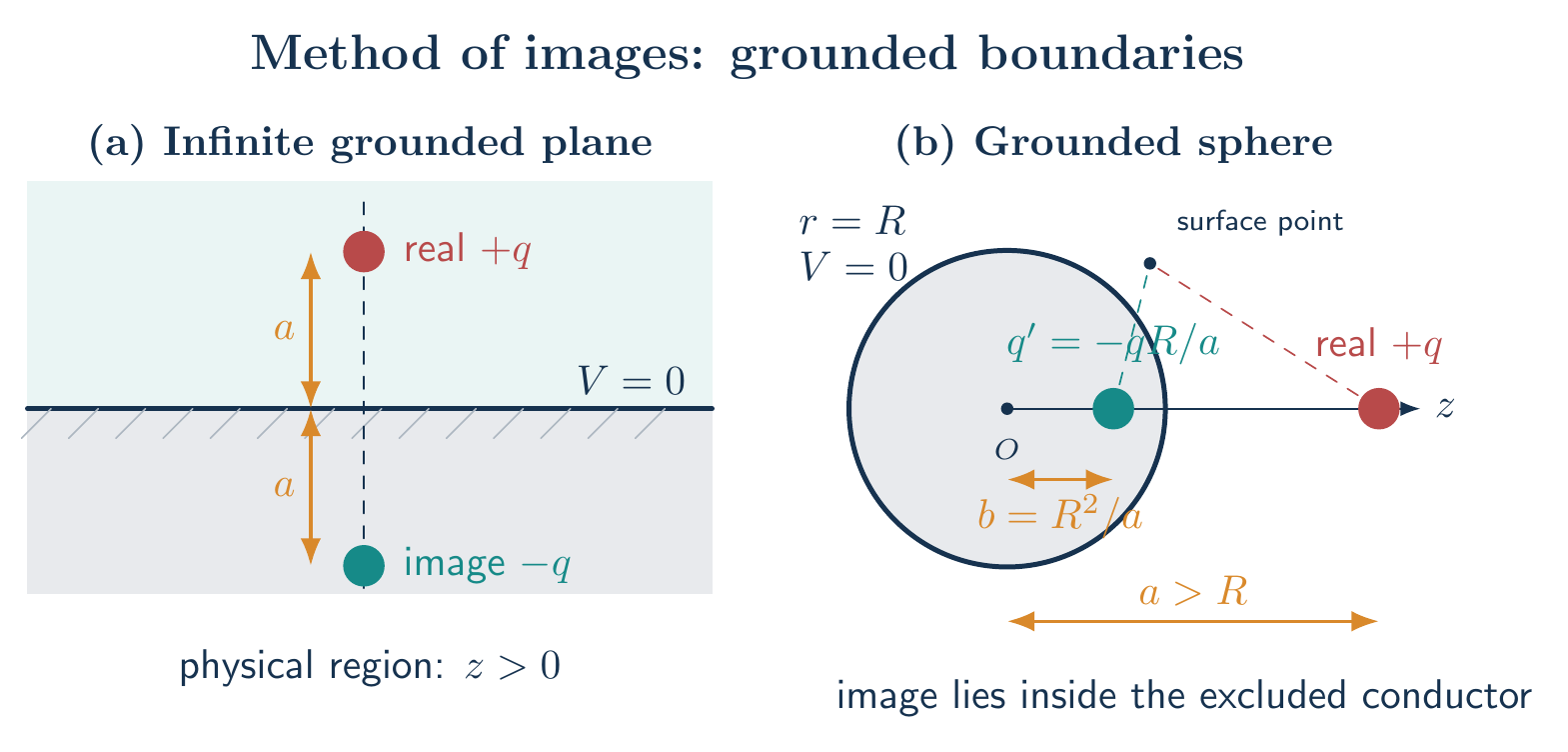
Place $q$ at $(0,0,a)$, where $a>0$, above the grounded conducting plane $z=0$. In the physical region $z>0$, replace the conductor by the image charge $-q$ at $(0,0,-a)$:

\[\boxed{ V(\rho,z)=\frac{q}{4\pi\epsilon_0} \left[ \frac{1}{\sqrt{\rho^2+(z-a)^2}} -\frac{1}{\sqrt{\rho^2+(z+a)^2}} \right]},\qquad z>0.\]

At $z=0$, the two distances are equal, so $V=0$. The potential also vanishes at infinity and has the correct singularity at $q$; uniqueness makes it the physical solution.

The induced surface charge follows from $\sigma=\epsilon_0E_z(0^+)=-\epsilon_0\left.\dfrac{\partial V}{\partial z}\right\rvert_{0^+}$:

\[\boxed{\sigma(\rho) =-\frac{qa}{2\pi(\rho^2+a^2)^{3/2}}}.\]

Indeed,

\[\int_0^\infty\sigma(\rho)\,2\pi\rho\,\mathrm d\rho=-q.\]

The field acting on the real charge equals the image field at its position. Their separation is $2a$, so

\[\boxed{\mathbf F =-\frac{q^2}{16\pi\epsilon_0a^2}\hat{\mathbf z}}.\]

The image is a mathematical device: it lies outside the physical solution region and is not an additional physical charge.

Image charge for a grounded conducting sphere

Let a grounded sphere have radius $R$, centred at the origin, and place $q$ at $z=a$, with $a>R$. Put

\[\boxed{q'=-\frac{R}{a}q}, \qquad \boxed{b=\frac{R^2}{a}}\]

at $z=b$, inside the sphere. For a point on $r=R$,

\[s^2=a^2+R^2-2aR\cos\theta\]

is its squared distance from $q$, while

\[s'^2=b^2+R^2-2bR\cos\theta =\frac{R^2}{a^2}s^2.\]

Thus $s’=(R/a)s$, and

\[\frac{q}{s}+\frac{q'}{s'} =\frac{q}{s}-\frac{Rq/a}{(R/a)s}=0.\]

Hence the unique exterior potential is

\[\boxed{ V(\mathbf r)=\frac{1}{4\pi\epsilon_0} \left( \frac{q}{\lvert\mathbf r-a\hat{\mathbf z}\rvert} +\frac{q'}{\lvert\mathbf r-b\hat{\mathbf z}\rvert} \right)},\qquad r\ge R.\]

Differentiation at $r=R$ gives

\[\boxed{ \sigma(\theta) =-\frac{q(a^2-R^2)} {4\pi R\left(a^2+R^2-2aR\cos\theta\right)^{3/2}}}.\]

Its integral is $q’=-qR/a$, as required by the far field. The attraction on $q$ is

\[\boxed{ \mathbf F =-\frac{q^2Ra} {4\pi\epsilon_0(a^2-R^2)^2}\hat{\mathbf z}}.\]

These results apply to a grounded sphere. For an isolated neutral sphere, a second image $+qR/a$ at the centre enforces zero total induced charge; changing the boundary condition changes the solution.

The dashed conductor boundaries enclose the fictitious images, while the real charges remain in the physical regions where the image potentials solve Laplace's equation.

The plane boundary, sphere-distance identity, induced-charge integrals, and force simplifications are verified with exact zero residuals in the Unit I image-method worksheet.

References

- Method of image charges: Wikipedia
- David J. Griffiths, Introduction to Electrodynamics, 4th ed., Cambridge University Press, 2017.
- William R. Smythe, Static and Dynamic Electricity, 3rd ed., McGraw-Hill, 1968.
- Edward M. Purcell and David J. Morin, Electricity and Magnetism, 3rd ed., Cambridge University Press, 2013.