27 May 2025

Electric Dipole and Quadrupole Fields

Far-field multipole expansion and the potentials and electric fields of electric dipoles and axial quadrupoles.

electricity-and-magnetism electrostatics electric-dipole electric-quadrupole

For localized point charges $q_a$ at positions $\mathbf r’_a$,

\[V(\mathbf r)=\frac{1}{4\pi\epsilon_0} \sum_a\frac{q_a}{\lvert\mathbf r-\mathbf r'_a\rvert}.\]

When $r\gg r’_a$, put $u=r’_a/r$ and let $\gamma_a$ be the angle between $\mathbf r$ and $\mathbf r’_a$. Then

\[\frac{1}{\lvert\mathbf r-\mathbf r'_a\rvert} =\frac{1}{r}\left(1-2u\cos\gamma_a+u^2\right)^{-1/2}.\]

Keeping terms through $u^2$,

\[\frac{1}{\lvert\mathbf r-\mathbf r'_a\rvert} =\frac{1}{r} +\frac{r'_a\cos\gamma_a}{r^2} +\frac{r_a'^2}{2r^3}\left(3\cos^2\gamma_a-1\right) +O(r^{-4}).\]

Thus the first three contributions are the monopole, dipole, and quadrupole potentials:

\[V(\mathbf r)=\frac{1}{4\pi\epsilon_0} \left[ \frac{Q}{r} +\frac{\mathbf p\cdot\hat{\mathbf r}}{r^2} +\frac{1}{2r^3}\sum_{i,j}Q_{ij}\hat r_i\hat r_j +\cdots \right],\]

where

\[Q=\sum_aq_a,\qquad \mathbf p=\sum_aq_a\mathbf r'_a,\]

and, with the traceless convention,

\[Q_{ij}=\sum_aq_a \left(3x'_{a,i}x'_{a,j}-r_a'^2\delta_{ij}\right).\]

The dipole moment has SI unit $\mathrm{C\,m}$, and $Q_{ij}$ has unit $\mathrm{C\,m^2}$.

Electric dipole

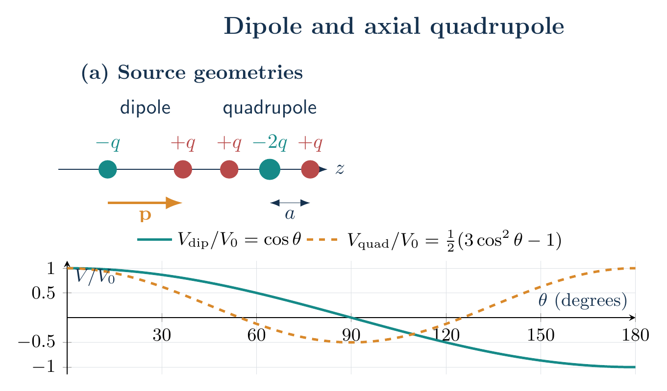
Place $-q$ and $+q$ a distance $d$ apart, and let $\mathbf d$ point from $-q$ to $+q$. The dipole moment is

\[\mathbf p=q\mathbf d.\]

The total charge is zero, so the leading far-field potential is

\[\boxed{V_{\mathrm{dip}}(\mathbf r) =\frac{1}{4\pi\epsilon_0} \frac{\mathbf p\cdot\hat{\mathbf r}}{r^2}}, \qquad r\gg d.\]

Choose $\mathbf p=p\hat{\mathbf z}$. Then

\[V_{\mathrm{dip}}(r,\theta) =\frac{p\cos\theta}{4\pi\epsilon_0r^2}.\]

In spherical coordinates,

\[E_r=-\frac{\partial V}{\partial r} =\frac{2p\cos\theta}{4\pi\epsilon_0r^3},\] \[E_\theta=-\frac{1}{r}\frac{\partial V}{\partial\theta} =\frac{p\sin\theta}{4\pi\epsilon_0r^3}, \qquad E_\phi=0.\]

Since $\mathbf p=p(\cos\theta\,\hat{\mathbf r}-\sin\theta\,\hat{\boldsymbol\theta})$, the two components combine to

\[\boxed{\mathbf E_{\mathrm{dip}}(\mathbf r) =\frac{1}{4\pi\epsilon_0r^3} \left[3(\mathbf p\cdot\hat{\mathbf r})\hat{\mathbf r}-\mathbf p\right]}.\]

On the axis $(\theta=0)$, $E=2p/(4\pi\epsilon_0r^3)$; on the equatorial plane $(\theta=\pi/2)$, the field has magnitude $p/(4\pi\epsilon_0r^3)$ and points opposite to $\mathbf p$.

Axial electric quadrupole

Take $+q$ at $z=\pm a$ and $-2q$ at the origin. Both $Q$ and $\mathbf p$ vanish. The second-order term from each outer charge is

\[\frac{1}{4\pi\epsilon_0} \frac{qa^2}{2r^3}\left(3\cos^2\theta-1\right).\]

Adding the two equal terms gives

\[\boxed{V_{\mathrm{quad}}(r,\theta) =\frac{qa^2}{4\pi\epsilon_0r^3} \left(3\cos^2\theta-1\right)}, \qquad r\gg a.\]

Let $A=qa^2/(4\pi\epsilon_0)$. Direct differentiation gives

\[E_r=-\frac{\partial}{\partial r} \left[\frac{A}{r^3}(3\cos^2\theta-1)\right] =\frac{3A}{r^4}(3\cos^2\theta-1),\]

and

\[E_\theta=-\frac{1}{r}\frac{\partial}{\partial\theta} \left[\frac{A}{r^3}(3\cos^2\theta-1)\right] =\frac{6A}{r^4}\sin\theta\cos\theta.\]

Therefore

\[\boxed{\mathbf E_{\mathrm{quad}} =\frac{qa^2}{4\pi\epsilon_0r^4} \left[ 3(3\cos^2\theta-1)\hat{\mathbf r} +6\sin\theta\cos\theta\,\hat{\boldsymbol\theta} \right]}.\]

The quadrupole potential decreases as $r^{-3}$, one power faster than the dipole potential.

The source geometries fix the signs; the curves plot $V_{\mathrm{dip}}/V_0=\cos\theta$ and $V_{\mathrm{quad}}/V_0=(3\cos^2\theta-1)/2$ at fixed radius.

The series coefficients and both field-component derivations are verified with exact zero residuals in the Unit I multipoles worksheet.

References

- Multipole expansion: Wikipedia
- David J. Griffiths, Introduction to Electrodynamics, 4th ed., Cambridge University Press, 2017.
- John D. Jackson, Classical Electrodynamics, 3rd ed., Wiley, 1998.
- Edward M. Purcell and David J. Morin, Electricity and Magnetism, 3rd ed., Cambridge University Press, 2013.