26 May 2025

Electric Flux, Gauss's Law, and Electrostatic Field Equations

Electric flux, integral and differential Gauss laws, symmetric applications, electrostatic potential, Poisson and Laplace equations, and uniqueness.

electricity-and-magnetism electrostatics gauss-law poisson-equation laplace-equation

Electric flux measures the component of an electric field that crosses an oriented surface. For

\[\mathrm d\mathbf a=\hat{\mathbf n}\,\mathrm da,\]

the flux element and total flux are

\[\mathrm d\Phi_E=\mathbf E\cdot\mathrm d\mathbf a, \qquad \Phi_E=\int_S\mathbf E\cdot\mathrm d\mathbf a.\]

In SI, $\mathbf E$ is measured in $\mathrm{N\,C^{-1}}$ and $\Phi_E$ in $\mathrm{N\,m^2\,C^{-1}}$.

Gauss’s law

For a point charge $q$, Coulomb’s law gives

\[\mathbf E(\mathbf r)=\frac{q}{4\pi\epsilon_0r^2}\hat{\mathbf r}.\]

At the charge, a surface element $\mathrm d\mathbf a$ subtends the signed solid angle

\[\mathrm d\Omega =\frac{\hat{\mathbf r}\cdot\mathrm d\mathbf a}{r^2}.\]

Therefore

\[\mathbf E\cdot\mathrm d\mathbf a =\frac{q}{4\pi\epsilon_0}\,\mathrm d\Omega.\]

A closed surface enclosing the charge subtends $4\pi$; one not enclosing it subtends zero net solid angle. Superposition over all charges, followed by the continuum limit, gives the integral law

\[\boxed{\oint_S\mathbf E\cdot\mathrm d\mathbf a =\frac{Q_{\mathrm{enc}}}{\epsilon_0}}, \qquad Q_{\mathrm{enc}}=\int_V\rho\,\mathrm d\tau .\]

Apply the divergence theorem:

\[\oint_S\mathbf E\cdot\mathrm d\mathbf a =\int_V\boldsymbol\nabla\cdot\mathbf E\,\mathrm d\tau =\frac{1}{\epsilon_0}\int_V\rho\,\mathrm d\tau .\]

Because the last equality holds for every volume,

\[\boxed{\boldsymbol\nabla\cdot\mathbf E=\frac{\rho}{\epsilon_0}}.\]

The integral form relates a field to enclosed charge; the differential form is the corresponding local statement.

Useful Gaussian surfaces follow the symmetry: cylinder for a line, pillbox for a sheet, and concentric sphere for spherical charge.

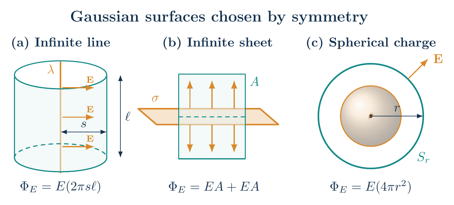
Symmetric applications

Infinite line charge

For line density $\lambda$, choose a coaxial cylinder of radius $s$ and length $\ell$. Cylindrical symmetry makes $\mathbf E=E(s)\hat{\mathbf s}$. The end-cap flux is zero and the curved-area flux is $E(2\pi s\ell)$. Thus

\[E(2\pi s\ell)=\frac{\lambda\ell}{\epsilon_0} \quad\Longrightarrow\quad \boxed{\mathbf E=\frac{\lambda}{2\pi\epsilon_0s}\hat{\mathbf s}}.\]

Infinite plane sheet

For surface density $\sigma$, reflection symmetry makes the fields on the two sides equal in magnitude and opposite in direction. A pillbox of face area $A$ gives

\[2EA=\frac{\sigma A}{\epsilon_0} \quad\Longrightarrow\quad \boxed{\mathbf E_{\pm}=\pm\frac{\sigma}{2\epsilon_0}\hat{\mathbf n}},\]

where $\hat{\mathbf n}$ points from the sheet toward the $+$ side.

Uniformly charged solid sphere

Let the sphere have radius $R$ and constant volume density $\rho$. A concentric Gaussian sphere of radius $r$ gives

\[E(r)\,4\pi r^2 =\frac{1}{\epsilon_0} \begin{cases} \rho\,4\pi r^3/3,&r<R,\\[2pt] \rho\,4\pi R^3/3,&r\ge R. \end{cases}\]

Hence

\[\boxed{\mathbf E(r)= \begin{cases} \dfrac{\rho r}{3\epsilon_0}\hat{\mathbf r},&r<R,\\[6pt] \dfrac{\rho R^3}{3\epsilon_0r^2}\hat{\mathbf r},&r\ge R. \end{cases}}\]

The two expressions agree at $r=R$, as they must because there is no separate surface charge there.

Conservative electrostatic field and potential

For stationary charges, Coulomb forces are conservative:

\[\oint_C\mathbf E\cdot\mathrm d\mathbf l=0.\]

Stokes’s theorem then gives

\[\int_S(\boldsymbol\nabla\times\mathbf E)\cdot\mathrm d\mathbf a=0 \quad\Longrightarrow\quad \boxed{\boldsymbol\nabla\times\mathbf E=0}.\]

Thus a single-valued scalar potential exists:

\[V(B)-V(A)=-\int_A^B\mathbf E\cdot\mathrm d\mathbf l, \qquad \boxed{\mathbf E=-\boldsymbol\nabla V}.\]

Substitution into the differential Gauss law yields

\[-\nabla^2V=\frac{\rho}{\epsilon_0}, \qquad \boxed{\nabla^2V=-\frac{\rho}{\epsilon_0}}\]

(Poisson’s equation). In a charge-free region,

\[\boxed{\nabla^2V=0}\]

(Laplace’s equation). Charge may still lie outside that region or on its boundary.

Uniqueness theorem

Suppose $V_1$ and $V_2$ satisfy the same Poisson equation in a volume and the same prescribed potential on its boundary. Their difference $U=V_1-V_2$ satisfies

\[\nabla^2U=0, \qquad \left.U\right\rvert_S=0.\]

Green’s first identity gives

\[\int_V\lvert\boldsymbol\nabla U\rvert^2\,\mathrm d\tau =\oint_S U\frac{\partial U}{\partial n}\,\mathrm da -\int_VU\nabla^2U\,\mathrm d\tau=0.\]

Both terms on the right vanish. Since the integrand on the left is non-negative, $\boldsymbol\nabla U=0$, so $U$ is constant. Its boundary value makes that constant zero. Therefore

\[\boxed{V_1=V_2}.\]

This Dirichlet theorem is why a correctly constructed image-charge potential is the physical solution. If instead the normal derivative is specified everywhere, the electric field is unique and the potential is unique up to an additive constant, provided the total-flux compatibility condition is satisfied.

The radial-field, Poisson, and Laplace identities are verified with exact residuals in the Unit I field-equations worksheet.

References

- Gauss’s law: Wikipedia
- David J. Griffiths, Introduction to Electrodynamics, 4th ed., Cambridge University Press, 2017.
- Edward M. Purcell and David J. Morin, Electricity and Magnetism, 3rd ed., Cambridge University Press, 2013.
- John R. Reitz, Frederick J. Milford, and Robert W. Christy, Foundations of Electromagnetic Theory, 4th ed., Addison-Wesley, 1993.