26 Jun 2025

Magnetic Properties of Matter

Magnetization, magnetic field intensity, susceptibility and permeability, magnetic classes, Langevin paramagnetism, hysteresis, and Quincke's method.

electricity-and-magnetism magnetization susceptibility hysteresis langevin-theory quincke-method

The magnetization is magnetic dipole moment per unit volume:

\[\boxed{\mathbf M =\frac{\text{magnetic dipole moment}}{\text{volume}}}.\]

Both $\mathbf M$ and magnetic field intensity $\mathbf H$ have SI unit $\mathrm{A\,m^{-1}}$; magnetic flux density $\mathbf B$ is measured in tesla.

Relations among $\mathbf B$, $\mathbf H$, and $\mathbf M$

A magnetization distribution is equivalent to the bound currents

\[\mathbf J_b=\boldsymbol\nabla\times\mathbf M, \qquad \mathbf K_b=\mathbf M\times\hat{\mathbf n}.\]

In magnetostatics,

\[\boldsymbol\nabla\times\mathbf B =\mu_0(\mathbf J_f+\mathbf J_b).\]

Substitute $\mathbf J_b=\boldsymbol\nabla\times\mathbf M$:

\[\boldsymbol\nabla\times \left(\frac{\mathbf B}{\mu_0}-\mathbf M\right) =\mathbf J_f.\]

This motivates

\[\boxed{\mathbf H=\frac{\mathbf B}{\mu_0}-\mathbf M}, \qquad \boxed{\mathbf B=\mu_0(\mathbf H+\mathbf M)}.\]

For a linear, isotropic material,

\[\boxed{\mathbf M=\chi_m\mathbf H},\]

where $\chi_m$ is the dimensionless magnetic susceptibility. Therefore

\[\mathbf B =\mu_0(1+\chi_m)\mathbf H =\mu\mathbf H =\mu_0\mu_r\mathbf H,\]

and

\[\boxed{\mu_r=1+\chi_m}, \qquad \boxed{\mu=\mu_0\mu_r}.\]

These proportionalities do not describe a ferromagnet throughout a hysteresis cycle because its response is nonlinear and history dependent.

Diamagnetic, paramagnetic, and ferromagnetic matter

Class	Susceptibility and response	Microscopic origin	Typical field removal
Diamagnetic	small $\chi_m<0$, hence $\mu_r<1$	field-induced moments oppose the applied field	induced magnetization disappears
Paramagnetic	small $\chi_m>0$, hence $\mu_r>1$	permanent atomic moments align partially against thermal disorder	alignment disappears
Ferromagnetic	large, nonlinear response	cooperative domain alignment	remanent magnetization can remain

Diamagnetism is weak and only mildly temperature dependent. Classical paramagnetism follows Curie’s $1/T$ law in the dilute weak-field limit. Ferromagnetic domains produce saturation and hysteresis.

Langevin theory of paramagnetism

Consider $N$ noninteracting classical dipoles per unit volume, each of fixed magnitude $m$. In a field $\mathbf B=B\hat{\mathbf z}$, a dipole at polar angle $\theta$ has energy

\[U=-mB\cos\theta.\]

Define

\[x=\frac{mB}{k_BT}.\]

The orientational Boltzmann factor is $e^{x\cos\theta}$. The azimuthal integral cancels in the average, so

\[\langle\cos\theta\rangle =\frac{\displaystyle\int_0^\pi \cos\theta\,e^{x\cos\theta}\sin\theta\,\mathrm d\theta} {\displaystyle\int_0^\pi e^{x\cos\theta}\sin\theta\,\mathrm d\theta}.\]

Put $u=\cos\theta$. The denominator is

\[Z(x)=\int_{-1}^{1}e^{xu}\,\mathrm du =\frac{e^x-e^{-x}}{x} =\frac{2\sinh x}{x}.\]

The numerator is $\mathrm dZ/\mathrm dx$. Hence

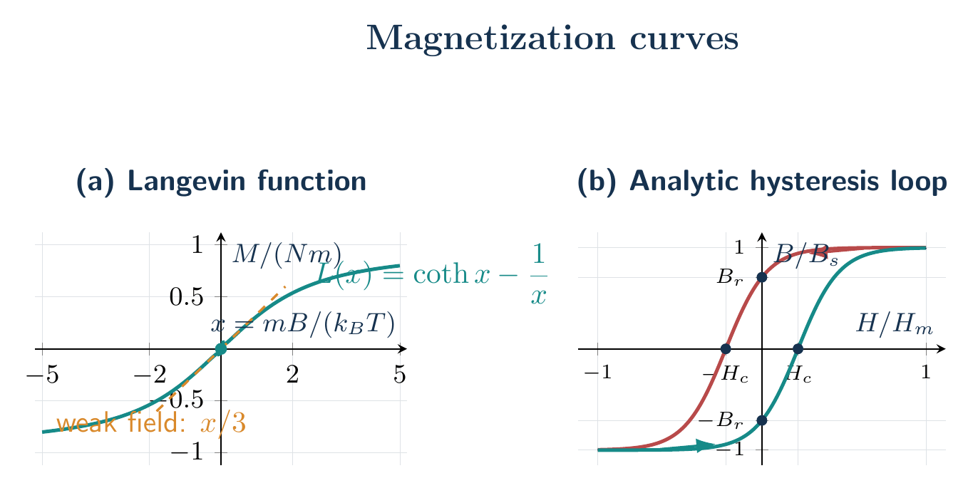
\[\langle\cos\theta\rangle =\frac{1}{Z}\frac{\mathrm dZ}{\mathrm dx} =\frac{\mathrm d}{\mathrm dx}\ln Z =\coth x-\frac{1}{x}.\]

Define the Langevin function

\[\boxed{L(x)=\coth x-\frac{1}{x}}.\]

The magnetization is therefore

\[\boxed{M=NmL(x)}.\]

For $x\ll1$,

\[\coth x=\frac{1}{x}+\frac{x}{3}-\frac{x^3}{45}+\cdots,\]

so

\[M\simeq Nm\frac{x}{3} =\frac{Nm^2B}{3k_BT}.\]

For a weak paramagnet, $\chi_m\ll1$, so $B\simeq\mu_0H$. Thus

\[M\simeq\frac{\mu_0Nm^2}{3k_BT}H\]

and

\[\boxed{\chi_m=\frac{\mu_0Nm^2}{3k_BT}=\frac{C}{T}}, \qquad C=\frac{\mu_0Nm^2}{3k_B}.\]

This is Curie’s law under the stated classical, noninteracting, weak-field approximation. As $x\to\infty$, $L(x)\to1$ and $M\to Nm$, the saturation magnetization.

$B$-$H$ curve and hysteresis

Starting from a demagnetized specimen, increasing $H$ traces the initial magnetization curve toward saturation. If $H$ is then cycled, $B$ lags and traces a closed loop:

• at $H=0$, the remaining flux density $B_r$ is the remanence;
• a reverse field of magnitude $H_c$ is required to make $B=0$; $H_c$ is the coercive field;
• at large $\lvert H\rvert$, the material approaches saturation.

The energy converted to heat per unit volume in one quasistatic cycle is the loop area:

\[\boxed{w_{\mathrm{hyst}}=\left\lvert\oint H\,\mathrm dB\right\rvert}.\]

Its unit is $\mathrm{A\,m^{-1}}\times\mathrm T=\mathrm{J\,m^{-3}}$. Soft magnetic materials have a narrow loop and low coercivity; hard magnetic materials have a wider loop and retain magnetization.

The Langevin curve approaches saturation smoothly. The analytic two-branch loop identifies $B_r$ and $H_c$ and illustrates the finite hysteresis area.

Measurement of susceptibility by Quincke’s method

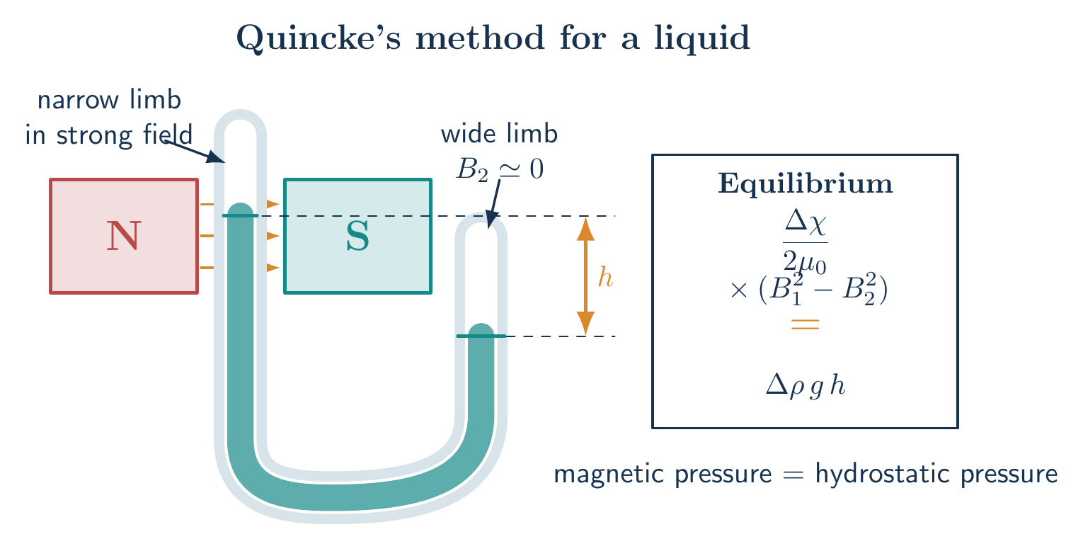
One limb of a Quincke tube is narrow and placed between magnet poles; the other limb is wide and nearly outside the field. For a weak linear liquid, the magnetic force density along $z$ is

\[f_z=\frac{\chi_m}{2\mu_0} \frac{\mathrm d(B^2)}{\mathrm dz}.\]

If the liquid and surrounding gas have susceptibility contrast

\[\Delta\chi=\chi_{\mathrm{liquid}}-\chi_{\mathrm{gas}},\]

integration over a column of cross-sectional area $A$, between fields $B_2$ and $B_1$, gives

\[F_m =A\int\frac{\Delta\chi}{2\mu_0}\,\mathrm d(B^2) =\frac{A\Delta\chi}{2\mu_0}(B_1^2-B_2^2).\]

At equilibrium this magnetic force is balanced by the hydrostatic force

\[F_g=A\,\Delta\rho\,g\,h,\]

where $\Delta\rho=\rho_{\mathrm{liquid}}-\rho_{\mathrm{gas}}$ and $h$ is the hydrostatic head between the two free surfaces. Cancelling $A$,

\[\boxed{ \Delta\chi =\frac{2\mu_0\Delta\rho\,g\,h}{B_1^2-B_2^2}}.\]

Usually $B_2$, $\rho_{\mathrm{gas}}$, and $\chi_{\mathrm{gas}}$ are negligible, giving

\[\boxed{\chi_m\simeq\frac{2\mu_0\rho gh}{B^2}}.\]

If a microscope records only the motion of the narrow meniscus, that motion equals $h$ only when the wide limb’s level change is negligible; otherwise the level changes of both limbs must be included. A paramagnetic liquid rises in the stronger-field limb $(\chi_m>0)$, while a diamagnetic liquid is depressed $(\chi_m<0)$.

The magnetic-pressure difference between the two menisci is balanced by the hydrostatic head $h$.

Solved Problems

1. Linear magnetic material inside a long solenoid

A long solenoid has $n$ turns per unit length and carries current $I$. Its core is a linear material of susceptibility $\chi_m$. Find $H,M$, and $B$.

Solution. Ampere’s law for $\mathbf H$ encloses only the free winding current, so

\[\boxed{H=nI}.\]

The linear constitutive law then gives

\[\boxed{M=\chi_mnI}.\]

Finally,

\[B=\mu_0(H+M) =\boxed{\mu_0(1+\chi_m)nI}.\]

Thus $H$ is fixed by free current, whereas $M$ describes the material response that changes $B$.

2. Power dissipated by hysteresis

A specimen traces a $B$-$H$ loop whose enclosed area is $A_{BH}=\lvert\oint H\,\mathrm dB\rvert$. If its volume is $\mathcal V$ and it is cycled at frequency $f$, find the average hysteresis power.

Solution. The loop area is energy dissipated per unit volume per cycle. Energy lost by the specimen in one cycle is therefore

\[W_{\mathrm{cycle}}=A_{BH}\mathcal V.\]

There are $f$ cycles each second, so

\[\boxed{P_{\mathrm{hyst}}=fA_{BH}\mathcal V}.\]

This explains why a narrow-loop soft magnetic core is preferred in an AC transformer.

Descriptive Questions

1. How do $\mathbf H$ and $\mathbf B$ separate free-current excitation from material response?
2. Why does classical Langevin paramagnetism approach Curie’s law only in the weak-field limit?
3. How do remanence and coercivity distinguish soft and hard magnetic materials?
4. Why does the liquid rise or fall in Quincke’s method according to the sign of susceptibility?

Numerical Problems

1. Susceptibility from magnetic-moment data

A specimen of volume $3.00\times10^{-6}\,\mathrm{m^3}$ has magnetic moment $2.40\times10^{-3}\,\mathrm{A\,m^2}$ in an applied field $H=2.00\times10^5\,\mathrm{A\,m^{-1}}$. Find $M$, $\chi_m$, and $\mu_r$, and classify the response.

Answer: $M=8.00\times10^2\,\mathrm{A\,m^{-1}}$, $\chi_m=4.00\times10^{-3}$, and $\mu_r=1.004$; the response is paramagnetic.

2. Curie-law temperature change

A paramagnet has $\chi_m=1.20\times10^{-3}$ at $300\,\mathrm K$. Find its susceptibility at $450\,\mathrm K$ in the Curie regime.

Answer: $\chi_m=8.00\times10^{-4}$.

3. Quincke susceptibility

A liquid of density $1000\,\mathrm{kg\,m^{-3}}$ rises by $4.00\,\mathrm{mm}$ in a field $B=0.800\,\mathrm T$. Neglect the field and density of the surrounding gas. Find $\chi_m$.

Answer: $\chi_m=1.54\times10^{-4}$.

4. Finite-field Langevin magnetization

A classical paramagnet has number density $N=5.00\times10^{27}\,\mathrm{m^{-3}}$, dipole moment $m=2.00\times10^{-23}\,\mathrm{A\,m^2}$, and Langevin parameter $x=1.50$. Use the full Langevin function to find $L(x)$ and $M$.

Answer: $L(1.50)=0.438$ and $M=4.38\times10^4\,\mathrm{A\,m^{-1}}$.

The symbolic solutions and all printed numerical answers are verified in the Unit II magnetic-matter worksheet.

References

1. Magnetization: Wikipedia
2. Charles Kittel, Introduction to Solid State Physics, 8th ed., Wiley, 2004.
3. Stephen Blundell, Magnetism in Condensed Matter, Oxford University Press, 2001.
4. D. C. Tayal, Electricity and Magnetism, Himalaya Publishing House.