19 Jul 2025

C. V. Raman and S. N. Bose

Inelastic light scattering and the statistical mechanics of indistinguishable bosons.

bsc semester-iv mj-5 indian-scientists raman-effect bose-einstein-statistics

C. V. Raman and inelastic light scattering

Raman and his collaborators, notably K. S. Krishnan, established in 1928 that monochromatic light scattered by a material contains weak lines at frequencies different from the incident frequency. Raman received the 1930 Nobel Prize in Physics for work on light scattering and discovery of the effect.

Let the incident photon frequency be $\nu_0$ and a molecular vibrational frequency be $\nu_m$. Energy conservation gives three possibilities:

• Rayleigh scattering: $\nu_s=\nu_0$;
• Stokes Raman scattering: $\nu_s=\nu_0-\nu_m$ as the molecule gains $h\nu_m$;
• anti-Stokes Raman scattering: $\nu_s=\nu_0+\nu_m$ as an initially excited molecule loses $h\nu_m$.

Thus the Raman shift

\[\Delta\tilde\nu=\frac{\nu_0-\nu_s}{c}\]

measures a molecular rotational or vibrational energy difference and is largely independent of the chosen excitation frequency.

When $\tilde\nu$ is reported in $\mathrm{cm^{-1}}$, the positive Stokes convention gives the molecular energy gain $\Delta E=hc\,\Delta\tilde\nu$. A vibration is Raman-active only if its normal coordinate changes the molecular polarizability; this is a different selection rule from infrared absorption. At thermal equilibrium the anti-Stokes line is normally weaker because its initial vibrational level is less populated. Neglecting instrumental response, a common approximation is

\[\frac{I_{\rm AS}}{I_{\rm S}} \simeq \left(\frac{\nu_0+\nu_m}{\nu_0-\nu_m}\right)^4 \exp\!\left(-\frac{h\nu_m}{k_BT}\right).\]

The exponential is a population ratio; the fourth-power factor comes from the frequency dependence of spontaneous Raman scattering.

Photon energy bookkeeping for Stokes and anti-Stokes Raman lines. A dashed virtual level is not a stationary molecular eigenstate.

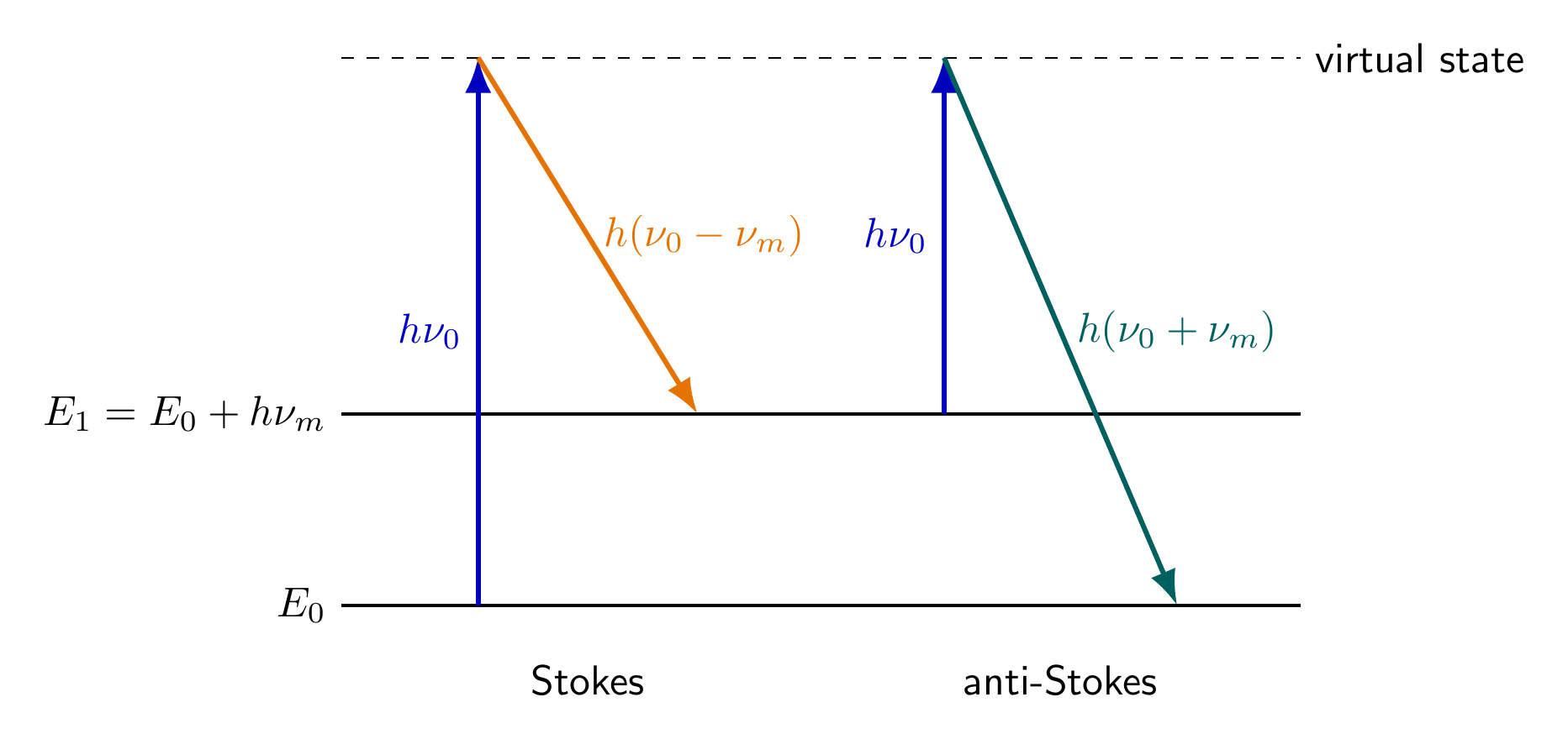
The editable source is raman-levels.tex. The discovery record is summarized by the Nobel Prize archive.

S. N. Bose and indistinguishable quanta

In 1924 Bose derived Planck’s radiation law by counting photon states without treating identical photons as individually labelled classical particles. Einstein translated the paper and extended the method to an ideal gas of material particles.

For bosons, any number $n_i=0,1,2,\ldots$ may occupy a one-particle state $i$. Maximizing entropy at fixed mean energy and particle number gives

\[\boxed{\bar n_i=\frac{1}{\exp[(\epsilon_i-\mu)/(k_BT)]-1}}.\]

This is the Bose-Einstein distribution. Photons have $\mu=0$ in thermal equilibrium because photon number is not fixed. Massive bosons can have conserved number; as $\mu$ approaches the ground-state energy, a macroscopic occupation of that state becomes possible, producing Bose-Einstein condensation.

For a finite occupation the denominator must remain positive, so $\mu<\epsilon_0$ before condensation, with $\epsilon_0$ the ground-state energy. The ideal distribution assumes thermal equilibrium, noninteracting particles and indistinguishable integer-spin quanta. Interactions can be weak enough for it to be a leading approximation, but they are not encoded in the displayed formula.

Classical Maxwell-Boltzmann statistics is recovered when $\exp[(\epsilon_i-\mu)/(k_BT)]\gg1$. Fermions instead obey the Pauli restriction and the plus-sign distribution. Bose’s decisive contribution was a new state-counting principle for indistinguishable quanta, not merely a correction to an old classical formula. The historical development is outlined by the American Physical Society.

The Maxima worksheet returns zero for Raman energy conservation and the algebraic Bose-factor identity.

Solved Problems

1. Stokes wavelength and molecular energy

A $532.0\ \mathrm{nm}$ laser produces a Stokes shift of $1000\ \mathrm{cm^{-1}}$. In wavenumbers,

\[\tilde\nu_0=\frac{1}{532.0\times10^{-7}\ \mathrm{cm}} =18796.99\ \mathrm{cm^{-1}}.\]

Hence

\[\tilde\nu_{\rm S}=18796.99-1000=17796.99\ \mathrm{cm^{-1}},\]

and

\[\lambda_{\rm S}=\frac{10^7}{17796.99}\ \mathrm{nm} =561.893\ \mathrm{nm}.\]

Using $hc=1.239841984\times10^{-4}\ \mathrm{eV\,cm}$,

\[\Delta E=hc(1000\ \mathrm{cm^{-1}})=0.123984\ \mathrm{eV}.\]

2. Thermal population behind an anti-Stokes line

For a $1000\ \mathrm{cm^{-1}}$ vibrational spacing at $300\ \mathrm{K}$, the excited-to-ground population ratio is

\[\frac{N_1}{N_0}\simeq \exp\!\left[-\frac{hc(1000\ \mathrm{cm^{-1}})}{k_B(300\ \mathrm{K})}\right].\]

With $hc/k_B=1.438776877\ \mathrm{K\,cm}$,

\[\frac{N_1}{N_0}=\exp(-4.79592)=8.263\times10^{-3}.\]

This is the Boltzmann population factor only; a predicted intensity ratio must also include the frequency and response factors stated above.

3. Occupation of a bosonic state

Let $\epsilon-\mu=2k_BT$. Substitution into the Bose–Einstein distribution gives

\[\bar n=\frac{1}{e^2-1}=0.1565.\]

The result is an ensemble mean, so it need not be an integer even though every individual occupation number is.

Descriptive Questions

1. Use energy conservation to distinguish Rayleigh, Stokes and anti-Stokes scattering.
2. Explain the physical origin of the temperature dependence of anti-Stokes intensity.
3. Which assumptions lead to the Bose–Einstein occupation factor, and why must $\mu<\epsilon_0$ above condensation?
4. What was conceptually new in Bose’s counting of radiation states?

Numerical Problems

1. A Stokes line at $560\ \mathrm{nm}$ carries $2.0\ \mathrm{\mu W}$. Find the photon rate using $N/t=P\lambda/(hc)$.

   Final answer: $5.64\times10^{12}\ \mathrm{s^{-1}}$.

2. For a uniform ideal three-dimensional Bose gas below $T_c$, use $N_0/N=1-(T/T_c)^{3/2}$ to find the condensate fraction at $T=0.50T_c$.

   Final answer: $N_0/N=0.646$.

3. At $(\epsilon-\mu)/(k_BT)=5$, by what percentage does the Bose occupation exceed the Maxwell–Boltzmann value $e^{-5}$?

   Final answer: $100[(1-e^{-5})^{-1}-1]=0.678\%$.

All conversions and rounded answers are verified in the Maxima worksheet.

References

1. Wikipedia overviews: Raman scattering and Bose–Einstein statistics.
2. Nobel Prize in Physics 1930: C. V. Raman.
3. American Physical Society: Bose, Einstein and the development of Bose–Einstein statistics.
4. Derek A. Long, The Raman Effect: A Unified Treatment of the Theory of Raman Scattering by Molecules, Wiley, 2002, Chapters 1–2.
5. R. K. Pathria and Paul D. Beale, Statistical Mechanics, 3rd ed., Elsevier, 2011, Chapter 7.