26 Jul 2025

Brownian Motion and Periodic Heat Flow

Brownian diffusion, rectilinear heat conduction in a metal rod, and the periodic-flow determination of conductivity.

bsc semester-iv mj-6 heat-and-thermodynamics brownian-motion thermal-conductivity

Brownian motion

A small particle suspended in a fluid receives rapidly fluctuating, unequal molecular impacts. Its visible irregular motion is Brownian motion. The mean displacement vanishes by isotropy,

\[\langle x\rangle=0,\]

but its mean-square displacement grows with time. For diffusion coefficient $D_B$,

\[\boxed{\langle x^2\rangle=2D_Bt}\]

in one dimension, and

\[\boxed{\langle r^2\rangle=6D_Bt}\]

in three dimensions.

These diffusion laws apply at times long compared with the particle’s velocity-relaxation time, when its detailed inertial motion has been averaged out.

Einstein’s fluctuation-dissipation relation is

\[\boxed{D_B=\frac{k_{\mathrm B}T}{\zeta}},\]

where $\zeta$ is the viscous drag coefficient. For a sphere of radius $a$ moving slowly in a continuum fluid of viscosity $\eta$, no-slip Stokes drag gives $\zeta=6\pi\eta a$, so

\[\boxed{D_B=\frac{k_{\mathrm B}T}{6\pi\eta a}}.\]

The dimensions are $[k_{\mathrm B}T/\zeta]=\mathrm{m^2\,s^{-1}}$. Brownian motion provided direct quantitative evidence for molecular agitation and permits measurements of molecular-scale constants through diffusion.

Rectilinear flow of heat in a metal rod

For one-dimensional heat flow along a uniform rod, Fourier’s law is

\[\boxed{\dot Q=-KA\frac{\partial T}{\partial x}},\]

where $K$ is thermal conductivity and $A$ is cross-sectional area. The minus sign makes heat flow toward decreasing temperature. In steady state with $T(0)=T_1$, $T(L)=T_2$, constant $K$, and no lateral heat loss,

\[T(x)=T_1-\frac{T_1-T_2}{L}x.\]

For $T_1>T_2$, the heat rate in the positive $x$ direction is

\[\boxed{\dot Q=KA\frac{T_1-T_2}{L}}.\]

For transient conduction, energy conservation on a slice $A\,dx$ gives

\[\rho cA\,dx\frac{\partial T}{\partial t} =KA\,dx\frac{\partial^2T}{\partial x^2},\]

where $\rho$ is mass density and $c$ is specific heat capacity. Thus

\[\boxed{\frac{\partial T}{\partial t} =\alpha\frac{\partial^2T}{\partial x^2}}, \qquad \boxed{\alpha=\frac{K}{\rho c}}.\]

$\alpha$ is thermal diffusivity with units $\mathrm{m^2\,s^{-1}}$.

Periodic flow method

Take a long uniform rod initially about mean temperature $T_0$. Drive its end periodically:

\[T(0,t)=T_0+A_0\cos\omega t,\]

and require the oscillation to remain bounded as $x\to\infty$. For $\theta=T-T_0$, use the complex trial form $\theta=\Re[A_0e^{i\omega t-kx}]$. Substitution into $\partial\theta/\partial t=\alpha\,\partial^2\theta/\partial x^2$ gives $\alpha k^2=i\omega$. The root with positive real part, required for decay as $x\to\infty$, is $k=(1+i)q$ with $q=\sqrt{\omega/(2\alpha)}$. Taking the real part gives

\[\boxed{\theta(x,t)=A_0e^{-qx}\cos(\omega t-qx)}, \qquad \boxed{q=\sqrt{\frac{\omega}{2\alpha}}}.\]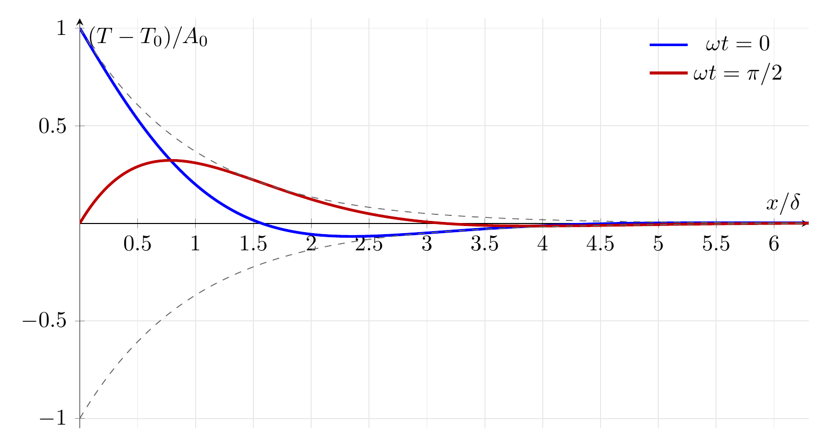

The amplitude decreases as $A(x)=A_0e^{-qx}$ and the phase lags by $qx$. At two positions $x_1<x_2$, let $\Delta x=x_2-x_1$, amplitudes be $A_1,A_2$, and the later temperature maximum lag by $\Delta t$. Then

\[q=\frac{\ln(A_1/A_2)}{\Delta x} =\frac{\omega\Delta t}{\Delta x}.\]

Since $\alpha=\omega/(2q^2)$ and the period is $P=2\pi/\omega$, the amplitude and phase measurements give independently

\[\boxed{\alpha =\frac{\pi(\Delta x)^2} {P[\ln(A_1/A_2)]^2}},\] \[\boxed{\alpha =\frac{P(\Delta x)^2}{4\pi(\Delta t)^2}}.\]

Finally,

\[\boxed{K=\rho c\alpha}.\]

The method assumes constant $K$, $\rho$, and $c$, one-dimensional conduction, a rod long compared with the penetration depth $1/q$, negligible or corrected lateral heat loss, and measurements taken after the initial transient has died away. The Unit III Maxima worksheet also verifies the periodic heat-wave differential-equation residual as zero.

References

- Brownian motion, Wikipedia.
- A. Einstein, Investigations on the Theory of the Brownian Movement, Dover, 1956, chapters 1-3.
- H. S. Carslaw and J. C. Jaeger, Conduction of Heat in Solids, 2nd ed., Oxford University Press, 1959, chapters 1-2.