

24 Jun 2025
Lagrangian Dynamics and Applications
Hamilton's principle, Euler-Lagrange equations, oscillators, uniform gravity, and electromagnetic coupling.
Lagrange’s equations
Suppose the generalized force is
\[Q_j=-\frac{\partial V}{\partial q_j}+Q_j^{(\mathrm{nc})},\]where $Q_j^{(\mathrm{nc})}$ contains any non-conservative part. With the Lagrangian $L=T-V$, D’Alembert’s equation becomes
\[\boxed{ \frac{d}{dt}\frac{\partial L}{\partial\dot q_j} -\frac{\partial L}{\partial q_j}=Q_j^{(\mathrm{nc})}}.\]For a conservative system, the right-hand side is zero. These are Lagrange’s equations, also called the Euler-Lagrange equations.
Hamilton’s principle
Let the action between two fixed times be
\[S[q]=\int_{t_1}^{t_2}L(q_i,\dot q_i,t)\,dt.\]Compare the physical path with $q_i(t,\epsilon)=q_i(t)+\epsilon\eta_i(t)$. The configuration endpoints are fixed:
\[\eta_i(t_1)=\eta_i(t_2)=0.\]The first variation is
\[\delta S =\int_{t_1}^{t_2}\sum_i\left( \frac{\partial L}{\partial q_i}\eta_i +\frac{\partial L}{\partial\dot q_i}\dot\eta_i \right)dt.\]Integrating the second term by parts gives
\[\delta S =\left[\sum_i\frac{\partial L}{\partial\dot q_i}\eta_i\right]_{t_1}^{t_2} +\int_{t_1}^{t_2}\sum_i\left[ \frac{\partial L}{\partial q_i} -\frac{d}{dt}\left(\frac{\partial L}{\partial\dot q_i}\right) \right]\eta_i\,dt.\]The endpoint term vanishes. Hamilton’s principle, $\delta S=0$ for arbitrary interior variations $\eta_i$, therefore yields the Euler-Lagrange equations.
One-dimensional simple harmonic oscillator
For a mass $m$ attached to a spring of force constant $k$,
\[L=\frac12m\dot x^2-\frac12kx^2.\]Since $\partial L/\partial\dot x=m\dot x$ and $\partial L/\partial x=-kx$,
\[m\ddot x+kx=0.\]Thus
\[x(t)=A\cos(\omega t+\delta), \qquad \boxed{\omega=\sqrt{\frac{k}{m}}},\]where $\omega$ has units $\mathrm{s^{-1}}$.
Falling body in uniform gravity
Take $y$ positive upward and choose $V=mgy$. Then
\[L=\frac12m\dot y^2-mgy.\]The Euler-Lagrange equation gives
\[m\ddot y+mg=0, \qquad \boxed{y(t)=y_0+v_{0y}t-\frac12gt^2}.\]The sign follows from the stated upward-positive convention.
Two coupled oscillators
Consider two equal masses and three equal springs, with $x_1$ and $x_2$ measured from equilibrium:
\[L=\frac m2(\dot x_1^2+\dot x_2^2) -\frac k2\left[x_1^2+(x_2-x_1)^2+x_2^2\right].\]Differentiation gives
\[m\ddot x_1+2kx_1-kx_2=0, \qquad m\ddot x_2+2kx_2-kx_1=0.\]For a normal mode $x_j=A_j e^{i\omega t}$,
\[\begin{pmatrix} 2k-m\omega^2&-k\\ -k&2k-m\omega^2 \end{pmatrix} \begin{pmatrix}A_1\\A_2\end{pmatrix}=0.\]A non-zero amplitude requires
\[(2k-m\omega^2)^2-k^2=0.\]The two modes are therefore
\[\boxed{\omega_1^2=\frac{k}{m},\quad(A_1,A_2)\propto(1,1)},\]and
\[\boxed{\omega_2^2=\frac{3k}{m},\quad(A_1,A_2)\propto(1,-1)}.\]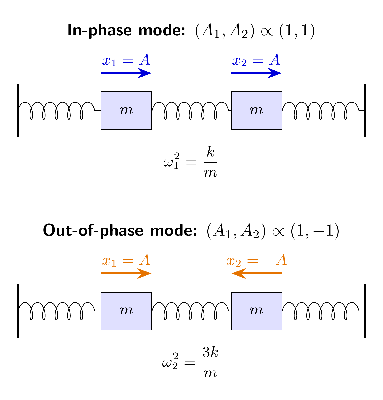
Charged particle in an electromagnetic field
Introduce scalar and vector potentials by
\[\mathbf E=-\nabla\phi-\frac{\partial\mathbf A}{\partial t}, \qquad \mathbf B=\nabla\times\mathbf A.\]The Lagrangian of a particle of charge $q$ is
\[\boxed{ L=\frac12m\dot{\mathbf r}^{\,2} +q\dot{\mathbf r}\cdot\mathbf A(\mathbf r,t) -q\phi(\mathbf r,t)}.\]For the Cartesian coordinate $x_i$,
\[\frac{\partial L}{\partial\dot x_i}=m\dot x_i+qA_i,\] \[\frac{d}{dt}\frac{\partial L}{\partial\dot x_i} =m\ddot x_i +q\frac{\partial A_i}{\partial t} +q\dot x_j\frac{\partial A_i}{\partial x_j},\]and
\[\frac{\partial L}{\partial x_i} =q\dot x_j\frac{\partial A_j}{\partial x_i} -q\frac{\partial\phi}{\partial x_i}.\]Repeated Cartesian indices are summed. The Euler-Lagrange equation becomes
\[m\ddot x_i =q\left[ -\frac{\partial\phi}{\partial x_i} -\frac{\partial A_i}{\partial t} +\dot x_j\left( \frac{\partial A_j}{\partial x_i} -\frac{\partial A_i}{\partial x_j} \right) \right].\]The last term is $(\dot{\mathbf r}\times\mathbf B)_i$, so
\[\boxed{m\ddot{\mathbf r}=q(\mathbf E+\dot{\mathbf r}\times\mathbf B)}.\]Maxima verification: coupled-mode eigenvalue residuals.
Solved Problems
1. Harmonic oscillator acted on by a constant force
A one-dimensional oscillator of mass $m$ and spring constant $k$ is also acted on by a constant force $F_0$ in the $+x$ direction. Find its motion for $x(0)=x_0$ and $\dot x(0)=v_0$.
The total potential and Lagrangian are
\[V(x)=\frac12kx^2-F_0x, \qquad L=\frac12m\dot x^2-\frac12kx^2+F_0x.\]The Euler-Lagrange equation is
\[\frac{d}{dt}(m\dot x)-(-kx+F_0)=0,\]so
\[m\ddot x+kx=F_0.\]The static equilibrium is $x_{\mathrm{eq}}=F_0/k$. With $y=x-x_{\mathrm{eq}}$,
\[m\ddot y+ky=0, \qquad \omega=\sqrt{\frac{k}{m}}.\]The initial data are $y(0)=x_0-F_0/k$ and $\dot y(0)=v_0$, giving
\[\boxed{ x(t)=\frac{F_0}{k} +\left(x_0-\frac{F_0}{k}\right)\cos\omega t +\frac{v_0}{\omega}\sin\omega t}.\]Completing the square,
\[V=\frac12k\left(x-\frac{F_0}{k}\right)^2-\frac{F_0^2}{2k},\]shows that the force shifts the equilibrium but does not change the angular frequency. As $F_0\to0$, the usual oscillator about $x=0$ is recovered.
2. Uniform magnetic field in the Landau gauge
For $\mathbf B=B\hat{\mathbf z}$, choose $\phi=0$ and $\mathbf A=Bx\hat{\mathbf y}$. Derive the planar equations of motion and identify the conserved canonical momentum.
Since
\[\nabla\times(Bx\hat{\mathbf y})=B\hat{\mathbf z},\]the Lagrangian is
\[L=\frac m2(\dot x^2+\dot y^2)+qBx\dot y.\]For $x$,
\[\frac{\partial L}{\partial\dot x}=m\dot x, \qquad \frac{\partial L}{\partial x}=qB\dot y,\]and therefore
\[\boxed{m\ddot x=qB\dot y}.\]For $y$,
\[\frac{\partial L}{\partial y}=0, \qquad \frac{\partial L}{\partial\dot y}=m\dot y+qBx.\]Thus $y$ is cyclic and
\[\boxed{p_y=m\dot y+qBx=\text{constant}}.\]Differentiating this constant gives
\[\boxed{m\ddot y=-qB\dot x}.\]Together these are precisely the Cartesian components of $m\ddot{\mathbf r}=q\dot{\mathbf r}\times\mathbf B$. The canonical momentum $p_y$ is gauge-dependent, but the mechanical momentum $m\dot y=p_y-qBx$ and the orbit are physical.
Descriptive Questions
- Derive Hamilton’s principle with fixed configuration endpoints and show explicitly how integration by parts produces the Euler-Lagrange equations.
- Explain why adding a total time derivative $dF(q,t)/dt$ to a Lagrangian leaves the equations of motion unchanged.
- Obtain the normal-coordinate eigenvalue equation for two coupled oscillators and explain the physical meaning of its eigenvectors.
- Derive the electromagnetic Lagrangian in scalar and vector potentials and distinguish canonical momentum from mechanical momentum.
Numerical Problems
- For $m=0.50\ \mathrm{kg}$, $k=8.0\ \mathrm{N\,m^{-1}}$, and $F_0=2.0\ \mathrm N$, find the shifted equilibrium, angular frequency, and period. Answer: $0.250\ \mathrm m$, $4.000\ \mathrm{s^{-1}}$, $1.571\ \mathrm s$.
- A body is projected upward from $y_0=20.0\ \mathrm m$ with $v_0=5.0\ \mathrm{m\,s^{-1}}$. With $y$ upward and $g=9.81\ \mathrm{m\,s^{-2}}$, find the time to reach the ground, the time to maximum height, and that height. Answer: $2.592\ \mathrm s$, $0.5097\ \mathrm s$, $21.274\ \mathrm m$.
- Two equal masses $m=0.20\ \mathrm{kg}$ are joined by three equal springs of constant $k=50\ \mathrm{N\,m^{-1}}$ in the arrangement derived above. Find both normal-mode angular frequencies. Answer: $15.811\ \mathrm{s^{-1}}$, $27.386\ \mathrm{s^{-1}}$.
- In the Landau gauge $\mathbf A=Bx\hat{\mathbf y}$, a particle has $m=0.050\ \mathrm{kg}$, $q=4.0\ \mathrm{mC}$, $B=0.80\ \mathrm T$, $x=0.15\ \mathrm m$, and $\dot y=2.0\ \mathrm{m\,s^{-1}}$. Find $m\dot y$, $qBx$, and $p_y$. Answer: $0.1000\ \mathrm{kg\,m\,s^{-1}}$, $4.800\times10^{-4}\ \mathrm{kg\,m\,s^{-1}}$, $0.10048\ \mathrm{kg\,m\,s^{-1}}$.
Maxima verification: shifted-oscillator and electromagnetic residuals, with all numerical values.
References
- Lagrangian mechanics — Wikipedia
- H. Goldstein, C. Poole, and J. Safko, Classical Mechanics, 3rd ed., Chapters 1–2, Pearson (2002).
- L. D. Landau and E. M. Lifshitz, Mechanics, 3rd ed., Sections 2–6, Butterworth-Heinemann (1976).
- J. R. Taylor, Classical Mechanics, Chapters 6–7, University Science Books (2005).


Discussion