22 Jun 2025

Euler and Fourth-Order Runge-Kutta Methods

numerical-methods ordinary-differential-equations euler-method runge-kutta

Consider the initial-value problem

\[\frac{dy}{dx}=f(x,y),\qquad y(x_0)=y_0.\]

A step method constructs $y_{n+1}$ at $x_{n+1}=x_n+h$ from information near $(x_n,y_n)$.

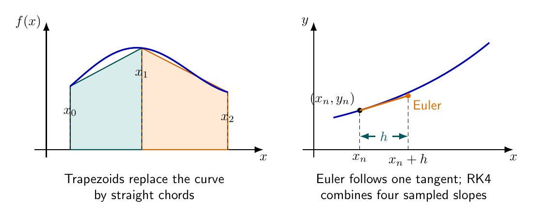
The figure is reproducible from its TikZ source.

Euler’s method

Taylor expansion gives

\[y(x_n+h)=y(x_n)+hy^{\prime}(x_n)+\frac{h^2}{2}y^{\prime\prime}(\xi_n).\]

Using $y^{\prime}=f(x,y)$ and dropping terms of order $h^2$ produces

\[\boxed{y_{n+1}=y_n+h f(x_n,y_n)}.\]

Thus Euler’s method follows the tangent at the start of each interval. Its local truncation error is $O(h^2)$; after roughly $(b-a)/h$ steps, these accumulated errors give global error $O(h)$.

Fourth-order Runge-Kutta method

RK4 samples four slopes:

\[k_1=h f(x_n,y_n),\] \[k_2=h f\left(x_n+\frac h2,y_n+\frac{k_1}{2}\right),\] \[k_3=h f\left(x_n+\frac h2,y_n+\frac{k_2}{2}\right),\] \[k_4=h f(x_n+h,y_n+k_3).\]

Their weighted combination is

\[\boxed{y_{n+1}=y_n+\frac{k_1+2k_2+2k_3+k_4}{6}}.\]

The weights are chosen to match the Taylor expansion through $h^4$. This can be seen directly for $y^{\prime}=y$:

\[k_1=hy,\] \[k_2=hy\left(1+\frac h2\right),\] \[k_3=hy\left(1+\frac h2+\frac{h^2}{4}\right),\] \[k_4=hy\left(1+h+\frac{h^2}{2}+\frac{h^3}{4}\right).\]

Substitution in the weighted update gives

\[y_{n+1}=y_n\left( 1+h+\frac{h^2}{2}+\frac{h^3}{6}+\frac{h^4}{24} \right),\]

which is the fourth-degree Taylor polynomial of $e^h$. For a smooth general equation, RK4 has local error $O(h^5)$ and global error $O(h^4)$.

One step for $y^{\prime}=y$

Let $y(0)=1$ and $h=0.1$. Euler gives

\[y_1^{\rm Euler}=1+0.1(1)=1.1.\]

For RK4,

\[k_1=0.1,\qquad k_2=0.105,\qquad k_3=0.10525,\qquad k_4=0.110525,\]

so

\[y_1^{\rm RK4} =1+\frac{0.1+2(0.105)+2(0.10525)+0.110525}{6} =1.105170833\ldots.\]

The exact value is $e^{0.1}=1.105170918\ldots$. The same step size therefore gives a visibly smaller RK4 error.

The symbolic expansion in the Maxima worksheet returns

rk4_residual = 0

where the residual is RK4 minus the fourth-degree Taylor update for $y^{\prime}=y$.

For the decay test equation $y^{\prime}=\lambda y$, Euler’s update is

\[y_{n+1}=(1+h\lambda)y_n.\]

When $\lambda<0$, numerical decay requires

\[\lvert1+h\lambda\rvert<1.\]

Thus consistency alone does not guarantee a useful computation: the chosen step must also lie in the method’s stability interval.

Solved Problems

1. Three Euler steps for exponential decay

Solve $y^{\prime}=-2y$, $y(0)=1$, using $h=0.1$ up to $x=0.3$. Euler’s formula becomes

\[y_{n+1}=y_n+0.1(-2y_n)=0.8y_n.\]

Therefore

\[y_1=0.8,\] \[y_2=0.8y_1=0.64,\] \[y_3=0.8y_2=0.512.\]

The exact value is

\[y(0.3)=e^{-0.6}\approx0.548811636,\]

so the signed global error is

\[y_3-y(0.3)\approx-0.036811636.\]

Euler underestimates the positive decaying solution here. The amplification factor $0.8$ satisfies $\lvert0.8\rvert<1$, so no spurious growth occurs.

2. One RK4 step for $y^{\prime}=x+y$

Let $y(0)=1$ and $h=0.2$. The four increments are

\[k_1=0.2(0+1)=0.2,\] \[k_2=0.2(0.1+1+0.1)=0.24,\] \[k_3=0.2(0.1+1+0.12)=0.244,\] \[k_4=0.2(0.2+1+0.244)=0.2888.\]

Hence

\[\begin{aligned} y_1&=1+\frac{0.2+2(0.24)+2(0.244)+0.2888}{6}\\ &=\boxed{1.2428}. \end{aligned}\]

Solving the linear equation analytically gives $y(x)=2e^x-x-1$, so

\[y(0.2)=1.242805516\ldots,\]

and the one-step signed error is $-5.516\times10^{-6}$. The error has the same unit as $y$.

Descriptive Questions

1. Derive Euler’s method from Taylor’s theorem and distinguish local from global truncation error.
2. State the four RK4 increments and explain the evaluation point used by each.
3. Show for $y^{\prime}=y$ that RK4 reproduces the exponential Taylor series through $h^4$.
4. Derive Euler’s stability condition for the decay equation $y^{\prime}=\lambda y$ with $\lambda<0$.

Numerical Problems

1. Use two Euler steps of size $h=0.25$ for $y^{\prime}=x$, $y(0)=0$, up to $x=0.5$. Answer: $y_1=0$, $y_2=0.0625$; exact $y(0.5)=0.125$, signed error $-0.0625$.

2. Apply one RK4 step of size $h$ to $y^{\prime}=1$ from $y(x_0)=y_0$. Answer: $k_1=k_2=k_3=k_4=h$, so $y_1=y_0+h$, exactly.

3. Find the Euler stability range for $y^{\prime}=-5y$. Answer: $\lvert1-5h\rvert<1$, hence $0<h<0.4$.

4. How many equal steps are required to integrate from $x=0$ to $x=2$ with $h=0.05$? Answer: $N=(2-0)/0.05=40$ steps.

The Euler sequences, RK4 increments, and stability arithmetic are checked in the Unit II Maxima worksheet; every displayed residual is zero.

References

1. Runge–Kutta methods — Wikipedia.
2. Richard L. Burden, J. Douglas Faires, and Annette M. Burden, Numerical Analysis, 10th ed., Chapter 5, “Initial-Value Problems for Ordinary Differential Equations.”
3. Steven C. Chapra and Raymond P. Canale, Numerical Methods for Engineers, 8th ed., Chapter 25, “Runge-Kutta Methods.”