21 Jun 2025

Trapezoidal, Simpson, and Gaussian Quadrature

numerical-methods quadrature trapezoidal-rule simpson-rule gaussian-quadrature

Numerical quadrature replaces

\[I=\int_a^b f(x)\,dx\]

by a weighted sum of sampled values. The weights follow by integrating an interpolating polynomial, rather than by guessing the area.

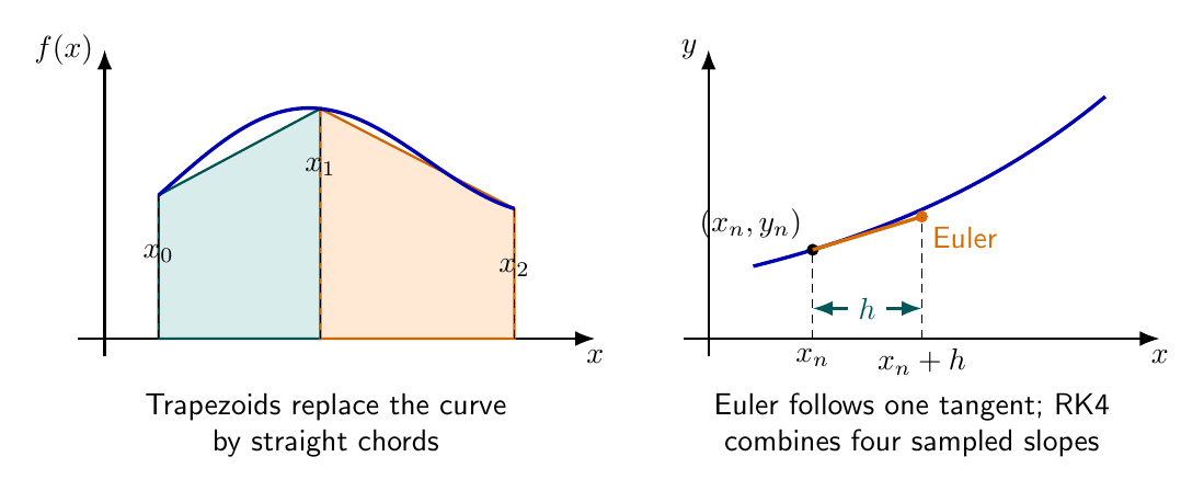
The construction is available as editable TikZ.

Trapezoidal rule

On $[x_i,x_{i+1}]$, where $h=x_{i+1}-x_i$, the linear interpolant is

\[P_1(x)=f_i\frac{x_{i+1}-x}{h} +f_{i+1}\frac{x-x_i}{h}.\]

Integrating both basis functions gives $h/2$, so

\[\int_{x_i}^{x_{i+1}}f(x)\,dx \approx\frac h2(f_i+f_{i+1}).\]

For $n$ equal subintervals, $x_i=a+ih$ and $h=(b-a)/n$. Adding adjacent panels yields the composite rule

\[\boxed{I_T=\frac h2\left[ f_0+2\sum_{i=1}^{n-1}f_i+f_n\right]}.\]

For a sufficiently smooth function,

\[I-I_T=-\frac{b-a}{12}h^2 f''(\xi),\]

for some $\xi\in(a,b)$. Halving $h$ therefore reduces the leading error by about a factor of four.

Simpson’s one-third rule

Use three equally spaced nodes $x_0,x_1,x_2$, with $x_1-x_0=x_2-x_1=h$, and put $t=(x-x_1)/h$. The nodes become $-1,0,1$, whose Lagrange basis polynomials are

\[L_{-1}(t)=\frac{t(t-1)}2,\qquad L_0(t)=1-t^2,\qquad L_1(t)=\frac{t(t+1)}2.\]

Their integrals from $-1$ to $1$ are $1/3,4/3,1/3$. Since $dx=h\,dt$,

\[\int_{x_0}^{x_2}f(x)\,dx \approx\frac h3(f_0+4f_1+f_2).\]

Adding pairs of panels gives, for even $n$,

\[\boxed{I_S=\frac h3\left[ f_0+f_n +4\sum_{\substack{i=1\\i\ {\rm odd}}}^{n-1}f_i +2\sum_{\substack{i=2\\i\ {\rm even}}}^{n-2}f_i \right]}.\]

The composite error is

\[I-I_S=-\frac{b-a}{180}h^4f^{(4)}(\xi).\]

Simpson’s rule is exact for every polynomial of degree at most three.

Two-point Gaussian quadrature

On $[-1,1]$, seek a symmetric two-point rule

\[\int_{-1}^{1}f(t)\,dt\approx w[f(-c)+f(c)].\]

Exactness for $f(t)=1$ requires $2w=2$, so $w=1$. Exactness for $f(t)=t^2$ then requires

\[2c^2=\int_{-1}^{1}t^2\,dt=\frac23,\]

which gives $c=1/\sqrt3$. Odd moments vanish by symmetry. Hence

\[\boxed{\int_{-1}^{1}f(t)\,dt \approx f\!\left(-\frac1{\sqrt3}\right) +f\!\left(\frac1{\sqrt3}\right)}\]

is exact through degree three. To integrate over $[a,b]$, use

\[x=\frac{a+b}{2}+\frac{b-a}{2}t,\qquad dx=\frac{b-a}{2}\,dt,\]

so

\[\boxed{\int_a^b f(x)\,dx\approx\frac{b-a}{2} \left[ f\!\left(\frac{a+b}{2}-\frac{b-a}{2\sqrt3}\right) +f\!\left(\frac{a+b}{2}+\frac{b-a}{2\sqrt3}\right) \right]}.\]

Exactness checks

For $f(x)=x^3-2x+4$ on $[0,2]$, Simpson’s rule with $h=1$ gives

\[I_S=\frac13[f(0)+4f(1)+f(2)] =\frac13(4+12+8)=8,\]

equal to the analytic integral. For $g(t)=t^2+2t+3$ on $[-1,1]$, the two-point Gaussian rule gives $20/3$, also exactly.

The Maxima worksheet displays

simpson_residual = 0
gauss_residual   = 0