

29 Jul 2025
Dielectric and Optical Properties
Polarization, local fields, Langevin-Debye theory, normal and anomalous dispersion, Cauchy and Sellmeier relations, complex permittivity, and optical attenuation.
Polarization is electric dipole moment per unit volume. In a linear isotropic dielectric,
\[\mathbf D=\epsilon_0\mathbf E+\mathbf P =\epsilon_0\epsilon_r\mathbf E,\]so
\[\boxed{\mathbf P=\epsilon_0(\epsilon_r-1)\mathbf E =\epsilon_0\chi_e\mathbf E}.\]$\mathbf P$ has unit $\mathrm{C\,m^{-2}}$; $\epsilon_r$ and $\chi_e$ are dimensionless.
Polarizability and local field
If one molecule develops dipole $\mathbf p=\alpha\mathbf E_{\rm loc}$, then $\alpha$ has unit $\mathrm{C\,m^2V^{-1}}$. For number density $N$,
\[\mathbf P=N\alpha\mathbf E_{\rm loc}.\]In an isotropic cubic dielectric, a spherical Lorentz cavity gives
\[\boxed{\mathbf E_{\rm loc}=\mathbf E+\frac{\mathbf P}{3\epsilon_0}}.\]Substitution yields
\[P=N\alpha\left(E+\frac{P}{3\epsilon_0}\right).\]Using $P=\epsilon_0(\epsilon_r-1)E$ and solving,
\[\boxed{\frac{\epsilon_r-1}{\epsilon_r+2} =\frac{N\alpha}{3\epsilon_0}},\]the Clausius-Mossotti relation.
Langevin-Debye equation
A permanent dipole $p_0$ at angle $\theta$ to the local field has energy
\[U=-p_0E_{\rm loc}\cos\theta.\]With $x=p_0E_{\rm loc}/(k_BT)$, its orientational partition integral is
\[Z=2\pi\int_0^\pi e^{x\cos\theta}\sin\theta\,d\theta =4\pi\frac{\sinh x}{x}.\]Therefore
\[\langle\cos\theta\rangle =\frac{d\ln Z}{dx}=\coth x-\frac1x\equiv L(x).\]For $x\ll1$, $L(x)=x/3+O(x^3)$, and
\[P_{\rm or}=Np_0L(x) \simeq\frac{Np_0^2}{3k_BT}E_{\rm loc}.\]If $\alpha_i$ is the induced electronic-plus-ionic polarizability, the effective weak-field polarizability is
\[\alpha=\alpha_i+\frac{p_0^2}{3k_BT}.\]The local-field result becomes the Langevin-Debye equation
\[\boxed{ \frac{\epsilon_r-1}{\epsilon_r+2} =\frac{N}{3\epsilon_0}\left(\alpha_i+\frac{p_0^2}{3k_BT}\right) }.\]Complex dielectric constant
Use the time convention $E(t)=\operatorname{Re}[E_0e^{-i\omega t}]$. A bound charge $q$ of mass $m$ obeys
\[m\ddot x+m\gamma\dot x+m\omega_0^2x=qE.\]For $x=x_0e^{-i\omega t}$,
\[x_0=\frac{qE_0/m}{\omega_0^2-\omega^2-i\gamma\omega}.\]With $N$ oscillators per unit volume and $P=Nqx$,
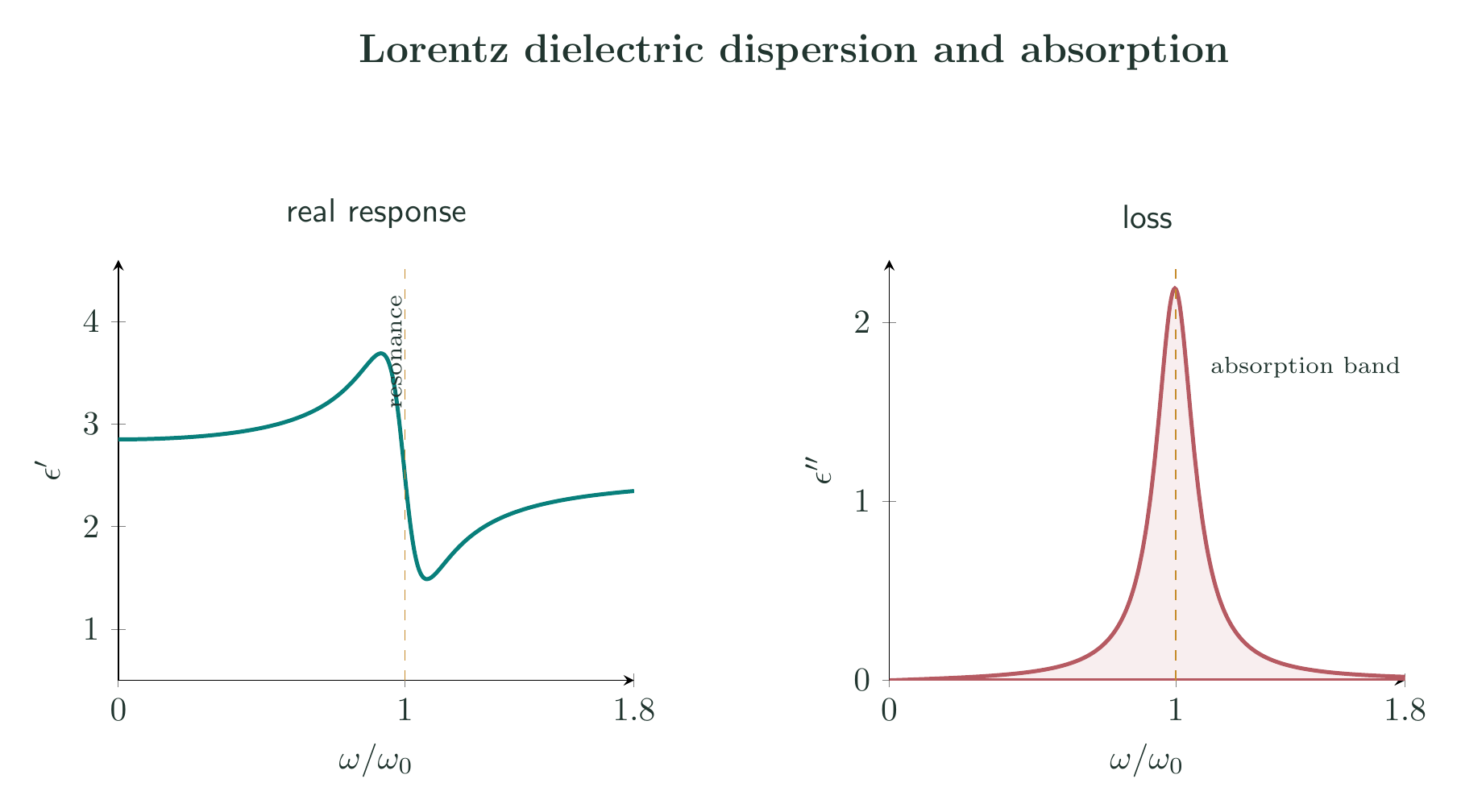
\[\boxed{ \epsilon_r(\omega)=\epsilon_\infty+ \frac{\Omega^2}{\omega_0^2-\omega^2-i\gamma\omega}}, \qquad \Omega^2=\frac{Nq^2}{\epsilon_0m}.\]Write $\epsilon_r=\epsilon^{\prime}+i\epsilon^{\prime\prime}$. Multiplying by the complex conjugate of the denominator gives
\[\boxed{ \epsilon^{\prime}=\epsilon_\infty+ \frac{\Omega^2(\omega_0^2-\omega^2)} {(\omega_0^2-\omega^2)^2+\gamma^2\omega^2}},\] \[\boxed{ \epsilon^{\prime\prime}=\frac{\Omega^2\gamma\omega} {(\omega_0^2-\omega^2)^2+\gamma^2\omega^2}}.\]$\epsilon^{\prime\prime}>0$ represents loss. The mean absorbed power density is
\[\boxed{\langle p\rangle=\frac12\omega\epsilon_0\epsilon^{\prime\prime}\lvert E_0\rvert^2}\]in $\mathrm{W\,m^{-3}}$.
Normal and anomalous dispersion
Away from resonance, damping is negligible and a transparent nonmagnetic material has $n^2\simeq\epsilon_r$. With several resonances,
\[n^2(\omega)=1+\sum_j\frac{A_j}{\omega_j^2-\omega^2}.\]Below a resonance, increasing $\omega$ normally increases $n$: $dn/d\omega>0$, equivalently $dn/d\lambda<0$. Close to an absorption resonance the slope can reverse, giving anomalous dispersion $dn/d\omega<0$.
Using $\omega=2\pi c/\lambda$ and defining $C_j=(2\pi c/\omega_j)^2$ gives the Sellmeier form
\[\boxed{n^2(\lambda)=1+\sum_j\frac{B_j\lambda^2}{\lambda^2-C_j}}.\]Far from resonance, $C_j/\lambda^2\ll1$ and
\[\frac{\lambda^2}{\lambda^2-C_j} =\frac1{1-C_j/\lambda^2} \simeq1+\frac{C_j}{\lambda^2}+\frac{C_j^2}{\lambda^4}+\cdots.\]Taking the square root and collecting constants produces Cauchy’s transparent-region relation
\[\boxed{n(\lambda)=A+\frac{B}{\lambda^2}+\frac{C}{\lambda^4}+\cdots}.\]Complex refractive index and extinction
Let the complex refractive index be
\[\widetilde n=n+i\kappa,\]where $\kappa$ is the extinction coefficient. For a nonmagnetic solid,
\[(n+i\kappa)^2=\epsilon^{\prime}+i\epsilon^{\prime\prime},\]so
\[\boxed{n^2-\kappa^2=\epsilon^{\prime}}, \qquad \boxed{2n\kappa=\epsilon^{\prime\prime}}.\]A wave propagating along $z$ contains
\[e^{i\widetilde n\omega z/c-i\omega t} =e^{-\kappa\omega z/c}e^{i(n\omega z/c-\omega t)}.\]Its intensity therefore obeys $I(z)=I_0e^{-\alpha z}$ with
\[\boxed{\alpha=\frac{2\omega\kappa}{c}=\frac{4\pi\kappa}{\lambda}}.\]At normal incidence from vacuum, the optical reflectance is
\[\boxed{R=\left\lvert\frac{\widetilde n-1}{\widetilde n+1}\right\rvert^2 =\frac{(n-1)^2+\kappa^2}{(n+1)^2+\kappa^2}}.\]Thus $n$ controls phase velocity and refraction, while $\kappa$ controls attenuation; both follow from the same complex dielectric response.
Solved Problems
1. Relative permittivity from molecular polarizability
For a cubic dielectric, the dimensionless combination $N\alpha/(3\epsilon_0)$ is $0.200$. Find $\epsilon_r$ using the Clausius–Mossotti relation.
Set
\[x=\frac{N\alpha}{3\epsilon_0}=0.200.\]Then
\[\frac{\epsilon_r-1}{\epsilon_r+2}=x.\]Cross-multiplication gives
\[\epsilon_r-1=x\epsilon_r+2x,\]so
\[\epsilon_r(1-x)=1+2x.\]Therefore
\[\boxed{\epsilon_r=\frac{1+2x}{1-x} =\frac{1.400}{0.800}=1.75}.\]Both $x$ and $\epsilon_r$ are dimensionless. The result satisfies $\epsilon_r\to1$ when $N\alpha\to0$. The pole at $x=1$ warns that the independent-polarizable-unit model cannot be continued without accounting for collective response.
2. Loss at a Lorentz resonance
A dielectric follows one Lorentz oscillator with $\epsilon_\infty=2.25$, $\Omega=1.00\times10^{15}\ \mathrm{s^{-1}}$, $\omega_0=2.00\times10^{15}\ \mathrm{s^{-1}}$, and $\gamma=1.00\times10^{14}\ \mathrm{s^{-1}}$. At resonance, find $\epsilon^{\prime}$ and $\epsilon^{\prime\prime}$, and find the mean absorbed power density for $\lvert E_0\rvert=100\ \mathrm{V\,m^{-1}}$.
At $\omega=\omega_0$, the dispersive numerator vanishes, so
\[\epsilon^{\prime}(\omega_0)=\epsilon_\infty=2.25.\]For the loss part,
\[\epsilon^{\prime\prime}(\omega_0) =\frac{\Omega^2\gamma\omega_0}{\gamma^2\omega_0^2} =\frac{\Omega^2}{\gamma\omega_0} =\frac{(1.00\times10^{15})^2} {(1.00\times10^{14})(2.00\times10^{15})} =5.00.\]With the $e^{-i\omega t}$ convention, positive $\epsilon^{\prime\prime}$ gives positive absorption:
\[\begin{aligned} \langle p\rangle &=\frac12\omega_0\epsilon_0\epsilon^{\prime\prime}\lvert E_0\rvert^2\\ &=\frac12(2.00\times10^{15})(8.854\times10^{-12}) (5.00)(100)^2\\ &=4.43\times10^8\ \mathrm{W\,m^{-3}}. \end{aligned}\]Thus
\[\boxed{\epsilon^{\prime}=2.25,\quad\epsilon^{\prime\prime}=5.00,\quad \langle p\rangle=4.43\times10^8\ \mathrm{W\,m^{-3}}}.\]The units are $(\mathrm{s^{-1}})(\mathrm{F\,m^{-1}})(\mathrm{V^2\,m^{-2}})=\mathrm{W\,m^{-3}}$. The absorbed power vanishes with the field amplitude, while decreasing $\gamma$ sharpens and raises the idealized resonance peak.
3. Optical constants from complex permittivity
At wavelength $600\ \mathrm{nm}$, a nonmagnetic material has $\epsilon^{\prime}=3.75$ and $\epsilon^{\prime\prime}=1.50$. Find $n$, $\kappa$, the absorption coefficient, and the intensity penetration depth $1/\alpha$.
Because
\[n^2-\kappa^2=\epsilon^{\prime}, \qquad 2n\kappa=\epsilon^{\prime\prime},\]squaring and adding gives
\[(n^2+\kappa^2)^2=(\epsilon^{\prime})^2+(\epsilon^{\prime\prime})^2.\]Choose the passive-medium branches $n>0$ and $\kappa>0$. With
\[\lvert\epsilon\rvert=\sqrt{(3.75)^2+(1.50)^2}=4.0389,\]we obtain
\[n=\sqrt{\frac{\lvert\epsilon\rvert+\epsilon^{\prime}}{2}} =1.973,\] \[\kappa=\sqrt{\frac{\lvert\epsilon\rvert-\epsilon^{\prime}}{2}} =0.3800.\]Therefore
\[\alpha=\frac{4\pi\kappa}{\lambda} =\frac{4\pi(0.3800)}{600\times10^{-9}} =7.96\times10^6\ \mathrm{m^{-1}},\]and
\[\boxed{n=1.973,\quad \kappa=0.3800,\quad \alpha=7.96\times10^6\ \mathrm{m^{-1}},\quad \alpha^{-1}=1.26\times10^{-7}\ \mathrm{m}}.\]$n$ and $\kappa$ are dimensionless, while $\alpha$ has inverse-length units. If $\epsilon^{\prime\prime}\to0^+$ with $\epsilon^{\prime}>0$, then $\kappa\to0$ and the absorption length diverges, as required for a transparent dielectric.
Descriptive Questions
- Derive the Lorentz local field and hence the Clausius–Mossotti relation for an isotropic cubic dielectric.
- Starting from the orientational partition function, obtain the Langevin–Debye equation and state its weak-field and temperature assumptions.
- Derive the real and imaginary parts of the Lorentz dielectric function for the $e^{-i\omega t}$ convention and explain normal and anomalous dispersion.
- Establish the relations among complex permittivity, complex refractive index, reflectance, and the intensity absorption coefficient.
Numerical Problems
-
A permanent molecular dipole is $3.00\ \mathrm{D}$ in a local field $1.00\times10^5\ \mathrm{V\,m^{-1}}$ at $300\ \mathrm{K}$. Check the weak-field condition and find $\langle\cos\theta\rangle$.
Answer: $x=p_0E/(k_BT)=2.42\times10^{-4}\ll1$ and $\langle\cos\theta\rangle\simeq x/3=8.05\times10^{-5}$.
-
At one frequency, $\epsilon^{\prime}=4.20$ and $\epsilon^{\prime\prime}=0.210$. Find the loss tangent and loss angle.
Answer: $\tan\delta=\epsilon^{\prime\prime}/\epsilon^{\prime}=0.0500$ and $\delta=2.86^\circ$.
-
Find the normal-incidence reflectance from vacuum for $n=1.80$ and $\kappa=0.120$.
Answer: \(R=\frac{(n-1)^2+\kappa^2}{(n+1)^2+\kappa^2}=0.0833,\) or $8.33\%$.
-
A transparent solid obeys $n=A+B/\lambda^2$ with $A=1.500$, $B=0.00400\ \mathrm{\mu m^2}$, and $\lambda$ in micrometres. Find $n$ at $0.500\ \mathrm{\mu m}$ and $0.700\ \mathrm{\mu m}$.
Answer: $n(0.500\ \mathrm{\mu m})=1.5160$ and $n(0.700\ \mathrm{\mu m})=1.50816$.
-
Find the cycle-averaged electric energy density \(u=\tfrac12\epsilon_0\epsilon_rE_{\rm rms}^2\) for a lossless dielectric with \(\epsilon_r=5.00\) and rms electric field \(E_{\rm rms}=2.00\times10^5\ \mathrm{V\,m^{-1}}\).
Answer: \(u=\tfrac12\epsilon_0\epsilon_rE_{\rm rms}^2=0.885\ \mathrm{J\,m^{-3}}\).
-
Find the phase velocity of light in a transparent nonmagnetic solid with refractive index $2.40$.
Answer: $v_p=c/n=1.25\times10^8\ \mathrm{m\,s^{-1}}$.
References
- Dielectric, Wikipedia
- Charles Kittel, Introduction to Solid State Physics, 8th ed., Chapters 15–16: “Optical Processes and Excitons” and “Dielectrics and Ferroelectrics.”
- David B. Tanner, Optical Effects in Solids, Cambridge University Press, 2019, Chapters 3–4: “The Complex Dielectric Function and Refractive Index” and “Classical Theories for the Dielectric Function.”
- MIT OpenCourseWare, 6.007 Electromagnetic Energy, lectures on the Lorentz oscillator and lossy electromagnetic waves


Discussion