29 Jun 2025

Free-Electron Theory of Metals

Drude-Lorentz transport, Sommerfeld statistics, Fermi energy, Fermi level, Fermi velocity, density of states, and thermal conductivity.

bsc semester-vi solid-state-physics free-electron-theory sommerfeld-model fermi-energy

The free-electron model replaces the detailed ionic potential inside a metal by a constant and treats collisions through a mean relaxation time. The classical Drude-Lorentz model explains Ohm’s law; Sommerfeld’s quantum statistics supplies the correct energy scale and thermal transport.

Drude-Lorentz electrical conductivity

Let $n$ be the conduction-electron number density, $m$ the electron mass, and $-e$ its charge. Between collisions an electric field accelerates an electron, while collisions relax its average velocity in time $\tau$:

\[m\frac{d\mathbf v_d}{dt}=-e\mathbf E-\frac{m\mathbf v_d}{\tau}.\]

In a static steady state, $d\mathbf v_d/dt=0$, so

\[\mathbf v_d=-\frac{e\tau}{m}\mathbf E.\]

The conventional current density is opposite to electron motion:

\[\mathbf j=-ne\mathbf v_d =\frac{ne^2\tau}{m}\mathbf E.\]

Thus

\[\boxed{\sigma=\frac{ne^2\tau}{m}}, \qquad \boxed{\rho=\frac{1}{\sigma}=\frac{m}{ne^2\tau}}.\]

$\sigma$ has SI unit $\mathrm{S\,m^{-1}}$ and $\rho$ has unit $\Omega\,\mathrm m$. The mean free path is $\ell=\bar v\tau$. The model attributes increasing resistivity to decreasing $\tau$, not to a change of electron charge or density.

For a harmonic field $\mathbf E=\operatorname{Re}[\mathbf E_0e^{-i\omega t}]$, take $\mathbf v_d=\operatorname{Re}[\mathbf v_0e^{-i\omega t}]$. The equation of motion gives

\[(-i\omega m+m/\tau)\mathbf v_0=-e\mathbf E_0,\]

and therefore

\[\boxed{\sigma(\omega)=\frac{ne^2\tau/m}{1-i\omega\tau}}.\]

Equivalently,

\[\sigma(\omega)=\sigma_0\frac{1+i\omega\tau}{1+(\omega\tau)^2} =\lvert\sigma(\omega)\rvert e^{i\phi}, \qquad \phi=\tan^{-1}(\omega\tau)>0.\]

The static result is recovered when $\omega\tau\ll1$. Under the stated $e^{-i\omega t}$ phasor convention, the positive phase means that the current leads the field by $\phi$.

Classical thermal conductivity

Electrons moving between regions of different temperature transport energy. The kinetic-theory form is

\[\boxed{\kappa=\frac13c_e\bar v^{\,2}\tau},\]

where $c_e$ is electron heat capacity per unit volume. Its unit is $\mathrm{W\,m^{-1}K^{-1}}$. Classical equipartition uses $c_e=3nk_B/2$ and $\bar v^{\,2}=3k_BT/m$, predicting an electronic heat capacity far larger than observed. This failure is removed by Fermi-Dirac statistics.

Sommerfeld theory and allowed states

Put the electrons in a cube of volume $V=L^3$ and impose periodic boundary conditions,

\[\psi(x+L,y,z)=\psi(x,y,z).\]

For $\psi\propto e^{i\mathbf k\cdot\mathbf r}$ this gives

\[k_x=\frac{2\pi n_x}{L},\quad k_y=\frac{2\pi n_y}{L},\quad k_z=\frac{2\pi n_z}{L}.\]

One $\mathbf k$ state occupies volume $(2\pi/L)^3$ in $k$ space and accepts two electrons of opposite spin. At $T=0$, states fill a sphere of radius $k_F$. Hence

\[N=2\frac{V}{(2\pi)^3}\frac{4\pi k_F^3}{3} =\frac{Vk_F^3}{3\pi^2}.\]

With $n=N/V$,

\[\boxed{k_F=(3\pi^2n)^{1/3}}.\]

For a free electron $E=\hbar^2k^2/(2m)$, so the highest occupied zero-temperature energy is

\[\boxed{E_F=\frac{\hbar^2}{2m}(3\pi^2n)^{2/3}}.\]

The corresponding Fermi speed and temperature are

\[\boxed{v_F=\frac{\hbar k_F}{m}=\sqrt{\frac{2E_F}{m}}}, \qquad \boxed{T_F=\frac{E_F}{k_B}}.\]

$E_F$ is measured in joules or electronvolts, $v_F$ in $\mathrm{m\,s^{-1}}$, and $T_F$ in kelvin.

Density of states

The number of spin states below wave number $k$ is

\[N(k)=\frac{Vk^3}{3\pi^2}.\]

Using $k=(2mE/\hbar^2)^{1/2}$,

\[N(E)=\frac{V}{3\pi^2}\left(\frac{2mE}{\hbar^2}\right)^{3/2}.\]

Differentiation gives the three-dimensional density of states

\[\boxed{ g(E)=\frac{dN}{dE} =\frac{V}{2\pi^2}\left(\frac{2m}{\hbar^2}\right)^{3/2}\sqrt E }.\]

It has unit $\mathrm{J^{-1}}$. At the Fermi energy,

\[\boxed{g(E_F)=\frac{3N}{2E_F}}.\]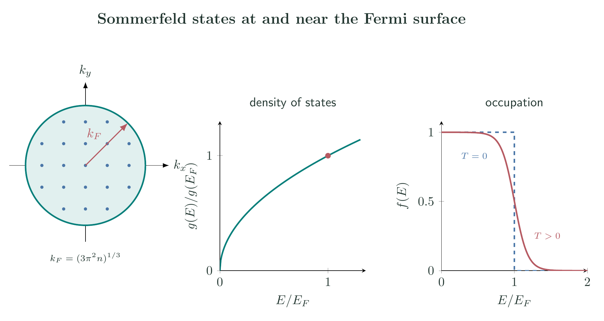

Periodic boundary conditions make the allowed $\mathbf k$ values uniformly spaced. Two spin states fill the Fermi sphere at $T=0$; $g(E)\propto\sqrt E$, while finite temperature rounds the occupation only within an energy of order $k_BT$ around the Fermi level.

Fermi level

At temperature $T$, the occupation probability is

\[\boxed{f(E)=\frac{1}{e^{(E-\mu)/k_BT}+1}},\]

where the chemical potential $\mu(T)$ is the Fermi level. Since $f(\mu)=1/2$, the Fermi level marks the midpoint of the occupation step. At $T=0$, $\mu=E_F$. For $k_BT\ll E_F$ at fixed density,

\[\mu(T)\simeq E_F\left[1-\frac{\pi^2}{12} \left(\frac{k_BT}{E_F}\right)^2\right].\]

Thus ordinary temperatures alter only electrons close to $E_F$; the deeply occupied states cannot change because nearby final states are already filled.

Sommerfeld heat and thermal conductivity

The low-temperature Sommerfeld result for electronic heat capacity is

\[\boxed{C_{V,e}=\frac{\pi^2}{2}Nk_B\frac{T}{T_F}}\]

or, per unit volume,

\[c_e=\frac{\pi^2}{2}nk_B^2\frac{T}{E_F}.\]

Only the fraction $T/T_F$ of electrons near the Fermi surface is thermally active. In the transport formula the active electrons move with approximately $v_F$, so

\[\begin{aligned} \kappa &=\frac13c_ev_F^2\tau\\ &=\frac13\left(\frac{\pi^2}{2}nk_B^2\frac{T}{E_F}\right) \left(\frac{2E_F}{m}\right)\tau\\ &=\boxed{\frac{\pi^2nk_B^2T\tau}{3m}}. \end{aligned}\]

Dividing by $\sigma T=(ne^2\tau/m)T$ eliminates $n,m,$ and $\tau$:

\[\boxed{ \frac{\kappa}{\sigma T}=L_0 =\frac{\pi^2}{3}\left(\frac{k_B}{e}\right)^2 }.\]

This is the Wiedemann-Franz law with Lorenz number $L_0\simeq2.44\times10^{-8}\ \mathrm{W\,\Omega\,K^{-2}}$. Its simple form assumes the same relaxation time governs charge and heat currents near the Fermi surface.

Solved Problems

1. Determine the Fermi scales from electron density

A monovalent metal has conduction-electron density $n=8.50\times10^{28}\ \mathrm{m^{-3}}$. Find $k_F$, $E_F$, $v_F$, and $T_F$ using $m=m_e$.

The occupied-state count gives

\[\begin{aligned} k_F &=(3\pi^2n)^{1/3}\\ &=\boxed{1.360\times10^{10}\ \mathrm{m^{-1}}}. \end{aligned}\]

Using $\hbar=1.054571817\times10^{-34}\ \mathrm{J\,s}$ and $m_e=9.1093837015\times10^{-31}\ \mathrm{kg}$,

\[\begin{aligned} E_F &=\frac{\hbar^2k_F^2}{2m_e} =1.1294\times10^{-18}\ \mathrm J\\ &=\boxed{7.049\ \mathrm{eV}},\\[4pt] v_F &=\frac{\hbar k_F}{m_e} =\boxed{1.575\times10^6\ \mathrm{m\,s^{-1}}},\\[4pt] T_F &=\frac{E_F}{k_B} =\boxed{8.180\times10^4\ \mathrm K}. \end{aligned}\]

The dimensional checks are $[k_F]=\mathrm{m^{-1}}$, $[\hbar^2k_F^2/m]=\mathrm J$, and $[\hbar k_F/m]=\mathrm{m\,s^{-1}}$. Since ordinary temperatures satisfy $T\ll T_F$, the gas is strongly degenerate, consistent with the Sommerfeld approximation.

2. Infer relaxation time and mean free path

For the same metal, take resistivity $\rho=1.70\times10^{-8}\ \Omega\,\mathrm m$. Find the Drude relaxation time and the Sommerfeld mean free path.

From $\rho=m/(ne^2\tau)$,

\[\begin{aligned} \tau &=\frac{m_e}{ne^2\rho}\\ &=\frac{9.1094\times10^{-31}} {(8.50\times10^{28})(1.60218\times10^{-19})^2(1.70\times10^{-8})}\\ &=\boxed{2.456\times10^{-14}\ \mathrm s}. \end{aligned}\]

The quantum model uses the speed of active electrons near the Fermi surface:

\[\ell=v_F\tau =(1.575\times10^6)(2.456\times10^{-14}) =\boxed{3.867\times10^{-8}\ \mathrm m=38.67\ \mathrm{nm}}.\]

The electron charge enters as $e^2$, so the conductivity is positive even though electron drift is opposite to $\mathbf E$. Dimensionally, $v_F\tau$ is a length; as $\rho\to0$ at fixed $n$, the model gives $\tau,\ell\to\infty$, its collisionless limit.

Descriptive Questions

1. How are the Drude dc and ac conductivities derived from the relaxation-time equation, including the current direction for negative carriers?
2. How does counting spin-degenerate states in a Fermi sphere yield $k_F$, $E_F$, and the three-dimensional density of states?
3. Why do only electrons within an energy of order $k_BT$ of $E_F$ contribute appreciably to low-temperature heat capacity?
4. How is the Wiedemann-Franz law derived, and under what assumptions is the Sommerfeld Lorenz number obtained?

Numerical Problems

1. A metal has $n=8.0\times10^{28}\ \mathrm{m^{-3}}$ and $E_F=7.0\ \mathrm{eV}$. Find its density of states per unit volume at $E_F$, expressed per electronvolt.

   Answer: $g(E_F)/V=1.714\times10^{28}\ \mathrm{eV^{-1}m^{-3}}$.

2. At $300\ \mathrm K$, find the Fermi-Dirac occupation of a state at $E=\mu+k_BT$.

   Answer: $f=1/(e+1)=0.268941$.

3. For $E_F=5.5\ \mathrm{eV}$ at $T=300\ \mathrm K$, estimate the low-temperature shift of the chemical potential.

   Answer: $E_F-\mu=9.99\times10^{-5}\ \mathrm{eV}$; $\mu\simeq5.499900\ \mathrm{eV}$.

4. For the Drude ac response with $\omega\tau=2$, find $\lvert\sigma(\omega)\rvert/\sigma_0$ and the current phase lead under the $e^{-i\omega t}$ convention.

   Answer: $1/\sqrt5=0.447214$; lead $\tan^{-1}2=63.435^\circ$.

5. Estimate the molar electronic heat capacity at $300\ \mathrm K$ for $E_F=7.0\ \mathrm{eV}$.

   Answer: $C_{V,e}=0.152\ \mathrm{J\,mol^{-1}K^{-1}}$.

6. Using the Sommerfeld Lorenz number, estimate $\kappa$ at $300\ \mathrm K$ for $\rho=1.70\times10^{-8}\ \Omega\,\mathrm m$.

   Answer: $\kappa=L_0T/\rho=431.1\ \mathrm{W\,m^{-1}K^{-1}}$.

Maxima verification worksheet

References

1. Free electron model.
2. Charles Kittel, Introduction to Solid State Physics, 8th ed., Chapter 6, Wiley.
3. Neil W. Ashcroft and N. David Mermin, Solid State Physics, Chapters 1–3, Holt, Rinehart and Winston.