30 Jul 2025

Magnetic Properties of Solids

Diamagnetism, classical and quantum paramagnetism, Curie and Weiss laws, ferro- and ferrimagnetic domains, and hysteresis loss.

bsc semester-vi solid-state-physics magnetism curie-law hysteresis

Magnetization $\mathbf M$ is magnetic dipole moment per unit volume, with unit $\mathrm{A\,m^{-1}}$. In an isotropic linear material,

\[\mathbf M=\chi_m\mathbf H, \qquad \mathbf B=\mu_0(\mathbf H+\mathbf M) =\mu_0(1+\chi_m)\mathbf H.\]

Diamagnets have $\chi_m<0$; paramagnets have small $\chi_m>0$; ferro- and ferrimagnets can retain a large magnetization after the applied field is removed.

Classical Langevin diamagnetism

An applied field $\mathbf B=B\hat z$ adds a Larmor angular velocity of magnitude $\omega_L=eB/(2m)$ to a bound electron orbit. The associated current change for one electron is

\[\Delta I=-\frac{e\omega_L}{2\pi}.\]

For an orbit of projected area $\pi r_\perp^2$, the induced moment is

\[\Delta\mu_z=\Delta I\,\pi r_\perp^2 =-\frac{e^2Br_\perp^2}{4m}.\]

The minus sign expresses Lenz’s law. For an isotropic atom,

\[\langle r_\perp^2\rangle =\langle x^2+y^2\rangle=\frac23\langle r^2\rangle.\]

If $N$ is the number of contributing electrons per unit volume and $B\simeq\mu_0H$ for weak response,

\[M=-\frac{Ne^2\langle r^2\rangle}{6m}B,\]

so

\[\boxed{\chi_{\rm dia}=-\frac{\mu_0Ne^2\langle r^2\rangle}{6m}}.\]

It is negative and approximately temperature independent.

Classical Langevin paramagnetism and Curie’s law

For permanent moments of magnitude $\mu$ in field $H$, the orientational energy is

\[U=-\mu B\cos\theta\simeq-\mu\mu_0H\cos\theta.\]

With $x=\mu\mu_0H/(k_BT)$, the Boltzmann average gives

\[\langle\cos\theta\rangle=\coth x-\frac1x=L(x),\]

and

\[\boxed{M=N\mu L(x)}.\]

For $x\ll1$, $L(x)\simeq x/3$, hence

\[M=\frac{N\mu^2\mu_0}{3k_BT}H,\]

and

\[\boxed{\chi_{\rm para}=\frac{C}{T}}, \qquad \boxed{C=\frac{\mu_0N\mu^2}{3k_B}}.\]

This is Curie’s law. Thermal disorder produces the inverse-temperature dependence.

Quantum paramagnetism

For total angular momentum $J$, the magnetic levels are

\[E_{m_J}=-g\mu_Bm_JB, \qquad m_J=-J,-J+1,\ldots,J.\]

Summing their Boltzmann weights gives

\[M=Ng\mu_BJ\,B_J(y), \qquad y=\frac{g\mu_BJ\mu_0H}{k_BT},\]

where

\[B_J(y)=\frac{2J+1}{2J}\coth\frac{(2J+1)y}{2J} -\frac1{2J}\coth\frac{y}{2J}.\]

For $y\ll1$,

\[B_J(y)\simeq\frac{J+1}{3J}y,\]

so

\[\boxed{ \chi=\frac{\mu_0N(g\mu_B)^2J(J+1)}{3k_BT} }.\]

The quantum result replaces the classical squared moment by $(g\mu_B)^2J(J+1)$.

Ferromagnetism, ferrimagnetism, and domains

Exchange interaction favours parallel moments in a ferromagnet, producing spontaneous magnetization below its Curie temperature. A macroscopic specimen divides into domains to reduce stray-field energy; moments are nearly parallel within each domain but different domains need not point alike. An applied field moves domain walls and rotates domain magnetizations.

In an antiferromagnet, neighbouring sublattices are antiparallel and equal, so the net moment vanishes. In a ferrimagnet they are antiparallel but unequal, leaving a nonzero net magnetization.

Weiss represents cooperative alignment by a molecular field

\[H_{\rm eff}=H+\lambda M.\]

Applying the Curie response to this field gives

\[M=\frac{C}{T}(H+\lambda M).\]

Therefore

\[M\left(1-\frac{C\lambda}{T}\right)=\frac{C}{T}H,\]

and

\[\boxed{\chi=\frac{M}{H}=\frac{C}{T-\Theta}}, \qquad \boxed{\Theta=C\lambda}.\]

This is the Curie-Weiss law above the ordering temperature. At $T=\Theta$, the linearized zero-field solution becomes unstable, signalling spontaneous order in the mean-field model.

B-H curve, hysteresis, and energy loss

Starting from a demagnetized specimen, increasing $H$ aligns domains until $B$ approaches saturation. On reducing $H$ to zero, a remanent flux density $B_r$ remains. A reverse coercive field $H_c$ is required to make $B=0$. Cycling the field traces a hysteresis loop because domain-wall motion is partly irreversible.

For a clean equation-generated sketch, the two branches may be parameterized by

\[M_\uparrow(H)=M_s\tanh\frac{H-H_c}{H_0}, \qquad M_\downarrow(H)=M_s\tanh\frac{H+H_c}{H_0},\]

with $B=\mu_0(H+M)$. This is a schematic loop, not a universal constitutive law.

Field-driven domain growth produces saturation and a history-dependent return path. The plotted branches use the displayed hyperbolic-tangent parameterization; the enclosed area represents dissipated energy per cycle.

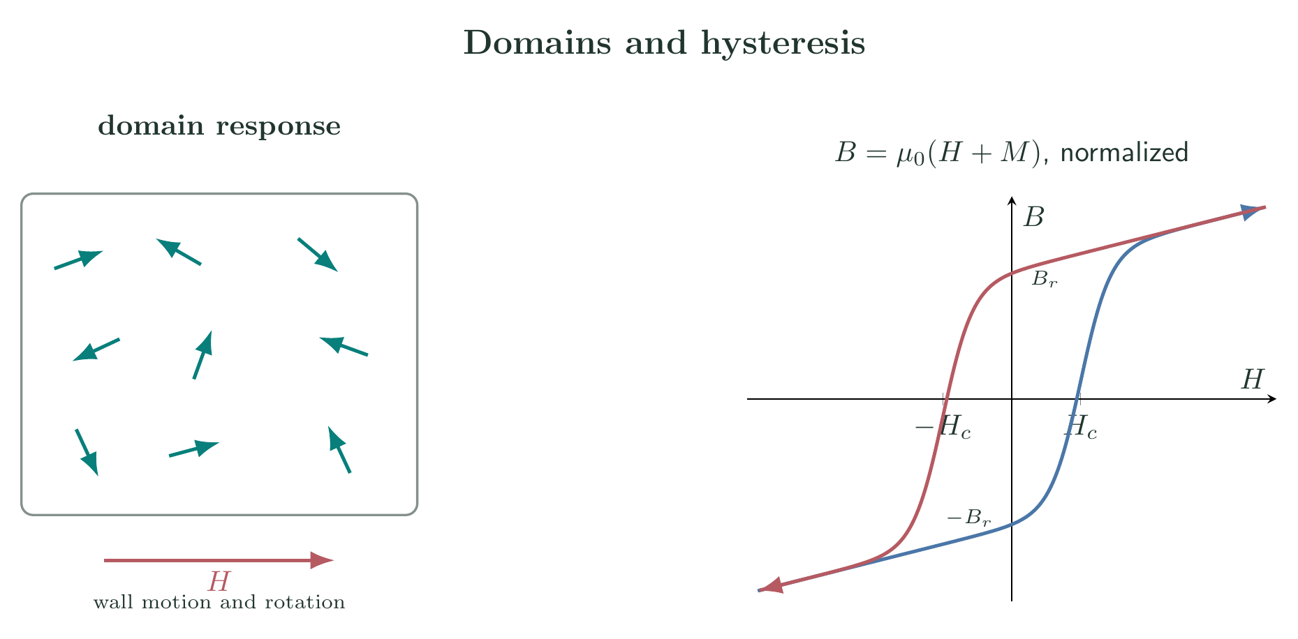
The magnetic work supplied per unit volume is $dW=H\,dB$. Over one complete cycle,

\[\boxed{W_{\rm loss}=\oint H\,dB},\]

which equals the loop area in the $B$-$H$ plane and has unit $\mathrm{J\,m^{-3}}$. Narrow loops reduce transformer-core loss; wide loops provide stable remanence in permanent magnets.

Maxima verification worksheet