14 May 2025

Radiation from Accelerated Charges and Antennas

Angular radiation from accelerated charges, oscillating dipoles, current elements, linear antennas, and coherent antenna arrays.

mj-16 radiation electric-dipole antenna antenna-array

The radiation part of the Liénard-Wiechert field is the term that decreases as $R^{-1}$:

\[\mathbf E_{\rm rad}=\frac{q}{4\pi\epsilon_0c} \left[ \frac{\mathbf n\times\{(\mathbf n-\boldsymbol\beta) \times\dot{\boldsymbol\beta}\}} {(1-\mathbf n\cdot\boldsymbol\beta)^3R} \right]_{t_r}, \qquad \mathbf B_{\rm rad}=\frac{1}{c}\mathbf n\times\mathbf E_{\rm rad}.\]

Both fields are transverse to $\mathbf n$. Their far-zone Poynting vector is

\[\mathbf S=\frac{1}{\mu_0}\mathbf E_{\rm rad}\times\mathbf B_{\rm rad} =\epsilon_0cE_{\rm rad}^2\mathbf n.\]

Because $dt=(1-\mathbf n\cdot\boldsymbol\beta)\,dt_r$, the energy crossing $R^2d\Omega$ during observer time $dt$ was emitted during $dt_r$. Hence

\[\boxed{ \frac{dP}{d\Omega} =\frac{q^2}{16\pi^2\epsilon_0c} \frac{\left\lvert\mathbf n\times[(\mathbf n-\boldsymbol\beta) \times\dot{\boldsymbol\beta}]\right\rvert^2} {(1-\mathbf n\cdot\boldsymbol\beta)^5}. }\]

Low- and high-velocity radiation

For $v\ll c$, put $\boldsymbol\beta=0$ and $\dot{\boldsymbol\beta}=\mathbf a/c$. If $\theta$ is the angle between $\mathbf a$ and $\mathbf n$,

\[\frac{dP}{d\Omega} =\frac{q^2a^2}{16\pi^2\epsilon_0c^3}\sin^2\theta.\]

Integration uses $d\Omega=2\pi\sin\theta\,d\theta$:

\[\begin{aligned} P&=\frac{q^2a^2}{16\pi^2\epsilon_0c^3} 2\pi\int_0^\pi\sin^3\theta\,d\theta\\ &=\frac{q^2a^2}{16\pi^2\epsilon_0c^3} 2\pi\left[\frac43\right] =\boxed{\frac{q^2a^2}{6\pi\epsilon_0c^3}}. \end{aligned}\]

This is the Larmor power. To perform the arbitrary-speed integral, choose $\boldsymbol\beta=\beta\hat{\mathbf z}$ and write $\mathbf a=a_\parallel\hat{\mathbf z}+a_\perp\hat{\mathbf x}$, $\mu=\cos\theta$, and $\mathbf n=(\sqrt{1-\mu^2}\cos\phi, \sqrt{1-\mu^2}\sin\phi,\mu)$. Since $\dot{\boldsymbol\beta}=\mathbf a/c$, the azimuthal average of the numerator is

\[\begin{aligned} &\frac1{2\pi}\int_0^{2\pi} \left\lvert\mathbf n\times[(\mathbf n-\boldsymbol\beta) \times\mathbf a]\right\rvert^2d\phi\\ &\qquad=a_\parallel^2(1-\mu^2) +\frac{a_\perp^2}{2} \left[(1+\beta^2)(1+\mu^2)-4\beta\mu\right]. \end{aligned}\]

Thus

\[P=\frac{q^2}{8\pi\epsilon_0c^3} \left(a_\parallel^2I_\parallel+a_\perp^2I_\perp\right),\]

where

\[I_\parallel=\int_{-1}^{1} \frac{1-\mu^2}{(1-\beta\mu)^5}\,d\mu,\] \[I_\perp=\frac12\int_{-1}^{1} \frac{(1+\beta^2)(1+\mu^2)-4\beta\mu} {(1-\beta\mu)^5}\,d\mu.\]

With $u=1-\beta\mu$, the limits become $1-\beta$ and $1+\beta$ and

\[\begin{aligned} I_\parallel &=\frac1{\beta^3}\int_{1-\beta}^{1+\beta} \frac{(\beta^2-1)+2u-u^2}{u^5}\,du =\frac4{3(1-\beta^2)^3}=\frac43\gamma^6,\\ I_\perp &=\frac1{2\beta^3}\int_{1-\beta}^{1+\beta} \frac{(1-\beta^2)^2-2(1-\beta^2)u+(1+\beta^2)u^2} {u^5}\,du\\ &=\frac4{3(1-\beta^2)^2}=\frac43\gamma^4. \end{aligned}\]

The $\beta\to0$ values follow continuously. Since $a^2-\lvert\boldsymbol\beta\times\mathbf a\rvert^2 =a_\parallel^2+(1-\beta^2)a_\perp^2$, the result is

\[\boxed{ P=\frac{q^2\gamma^6}{6\pi\epsilon_0c^3} \left[a^2-\lvert\boldsymbol\beta\times\mathbf a\rvert^2\right]. }\]

Thus $P=q^2\gamma^6a^2/(6\pi\epsilon_0c^3)$ for acceleration parallel to the velocity and $P=q^2\gamma^4a^2/(6\pi\epsilon_0c^3)$ for perpendicular acceleration.

Oscillating electric dipole

Let a localized source have dipole moment $\mathbf p(t)=p_0\cos\omega t\,\hat{\mathbf z}$ and size $d\ll\lambda$. In the radiation zone $r\gg\lambda$ its retarded vector potential is

\[\mathbf A(\mathbf r,t) =\frac{\mu_0}{4\pi r}\dot{\mathbf p}(t_r), \qquad t_r=t-\frac rc.\]

Keeping only derivatives of the retarded time, which supply the leading $r^{-1}$ fields,

\[\mathbf B_{\rm rad}=\nabla\times\mathbf A =-\frac{\mu_0}{4\pi cr} \mathbf n\times\ddot{\mathbf p}(t_r),\] \[\mathbf E_{\rm rad}=c\mathbf B_{\rm rad}\times\mathbf n =\frac{1}{4\pi\epsilon_0c^2r} \mathbf n\times[\mathbf n\times\ddot{\mathbf p}(t_r)].\]

Since $\lvert\ddot{\mathbf p}\rvert=\omega^2p_0\lvert\cos\omega t_r\rvert$,

\[\left\langle\frac{dP}{d\Omega}\right\rangle =\frac{p_0^2\omega^4}{32\pi^2\epsilon_0c^3}\sin^2\theta, \qquad \boxed{\langle P\rangle =\frac{p_0^2\omega^4}{12\pi\epsilon_0c^3}}.\]

The approximation requires source size $d\ll\lambda$, observation distance $r\gg\lambda$, and nonrelativistic source motion.

Small current element and linear antenna

A short element of length $\ell\ll\lambda$ carrying $I(t)=I_0\cos\omega t$ has charge amplitude $q_0=I_0/\omega$ by $I=dq/dt$, and dipole amplitude $p_0=q_0\ell=I_0\ell/\omega$. Therefore

\[\left\langle\frac{dP}{d\Omega}\right\rangle =\frac{I_0^2\ell^2\omega^2}{32\pi^2\epsilon_0c^3}\sin^2\theta =\frac{Z_0I_0^2(k\ell)^2}{32\pi^2}\sin^2\theta,\]

where $k=\omega/c$ and $Z_0=\sqrt{\mu_0/\epsilon_0}=\mu_0c$.

For a thin, centre-fed linear antenna of total length $L$ on the $z$-axis, take the standing current

\[I(z)=I_0\sin[k(L/2-\lvert z\rvert)],\qquad -L/2\le z\le L/2.\]

Far-zone contributions from $z$ acquire phase $e^{-ikz\cos\theta}$. Put $A=kL/2$, $\eta=\cos\theta$, and $u=kz$. Evenness of $I(z)$ cancels the imaginary part, so

\[\begin{aligned} \int_{-L/2}^{L/2}I(z)e^{-ikz\eta}\,dz &=\frac{2I_0}{k}\int_0^A\sin(A-u)\cos(\eta u)\,du\\ &=\frac{2I_0}{k}\int_0^A [\sin A\cos u-\cos A\sin u]\cos(\eta u)\,du\\ &=\frac{2I_0}{k} \frac{\cos(A\eta)-\cos A}{1-\eta^2}. \end{aligned}\]

The transverse projection supplies a factor $\sin\theta$. Apart from the common radial factor, the pattern amplitude is therefore

\[\boxed{ F(\theta)=\frac{2I_0}{k} \frac{\cos[(kL/2)\cos\theta]-\cos(kL/2)}{\sin\theta}. }\]

The displayed quotient has a removable axial limit. For $\theta\to0$, with $A=kL/2$,

\[\cos(A\cos\theta)-\cos A =\frac{A\sin A}{2}\theta^2+O(\theta^4), \qquad \sin\theta=\theta+O(\theta^3),\]

so $F(\theta)=(I_0A\sin A/k)\theta+O(\theta^3)\to0$; the $\theta\to\pi$ limit is likewise zero.

The radiation intensity is proportional to $\lvert F(\theta)\rvert^2$. For $L=\lambda/2$, this becomes $F(\theta)\propto\cos[(\pi/2)\cos\theta]/\sin\theta$.

Antenna arrays

For $N$ identical elements separated by $d$ along $z$, with phase advance $\delta$ between adjacent feeds, the phase step in direction $\theta$ is

\[\psi=kd\cos\theta+\delta.\]

The array factor is the geometric sum

\[\begin{aligned} AF&=\sum_{m=0}^{N-1}e^{im\psi} =\frac{1-e^{iN\psi}}{1-e^{i\psi}}\\ &=e^{i(N-1)\psi/2} \frac{\sin(N\psi/2)}{\sin(\psi/2)}. \end{aligned}\]

Thus

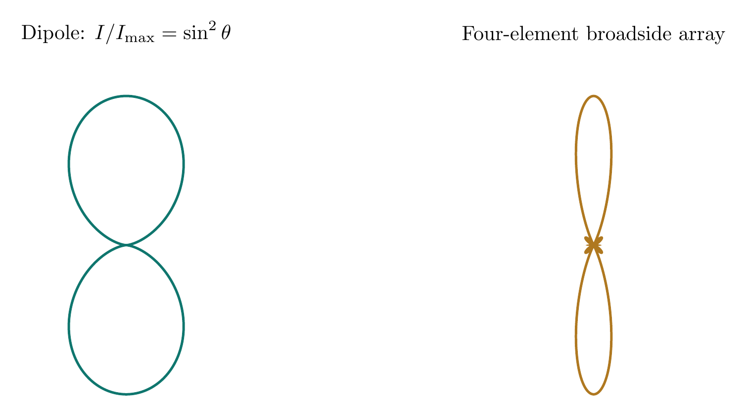
\[\boxed{\lvert AF\rvert^2=\left[\frac{\sin(N\psi/2)}{\sin(\psi/2)}\right]^2},\]

with the limiting value $N^2$ when $\psi=2m\pi$. The total pattern equals the single-element intensity multiplied by $\lvert AF\rvert^2$.

The dipole pattern follows \(\sin^2\theta\). The four-element broadside array uses \(d=\lambda/2\), \(\delta=0\), and the normalized factor \(\lvert AF/N\rvert^2\).

The angular integrals, Larmor limits, and array-factor identity are checked in the Maxima worksheet; every printed residual is zero.