

14 Jun 2025
Fourier Transforms, Delta Functions and Convolution
Fourier transforms of trigonometric, Gaussian, finite-train, and elementary functions, with derivative, inverse, delta, and convolution theorems.
Use the transform pair
\[\boxed{ F(k)=\int_{-\infty}^{\infty}f(x)e^{-ikx}\,dx, \qquad f(x)=\frac1{2\pi}\int_{-\infty}^{\infty}F(k)e^{ikx}\,dk. }\]The constants and signs in every formula below follow from this convention.
Dirac delta as a Fourier integral
The inverse transform of $F(k)=1$ defines
\[\boxed{ \delta(x-x_0)=\frac1{2\pi}\int_{-\infty}^{\infty} e^{ik(x-x_0)}\,dk. }\]This equality is distributional. Multiply by a smooth test function $g(x)$, integrate over $x$, and use the inverse transform to obtain $\int\delta(x-x_0)g(x)dx=g(x_0)$.
Trigonometric functions
Since
\[\int_{-\infty}^{\infty}e^{-i(k-k_0)x}\,dx =2\pi\delta(k-k_0),\]Euler’s relations give
\[\boxed{ \mathcal F\{\cos k_0x\} =\pi[\delta(k-k_0)+\delta(k+k_0)], }\] \[\boxed{ \mathcal F\{\sin k_0x\} =\frac\pi i[\delta(k-k_0)-\delta(k+k_0)]. }\]These transforms are distributions because an infinite sinusoid is not absolutely integrable.
Gaussian transform
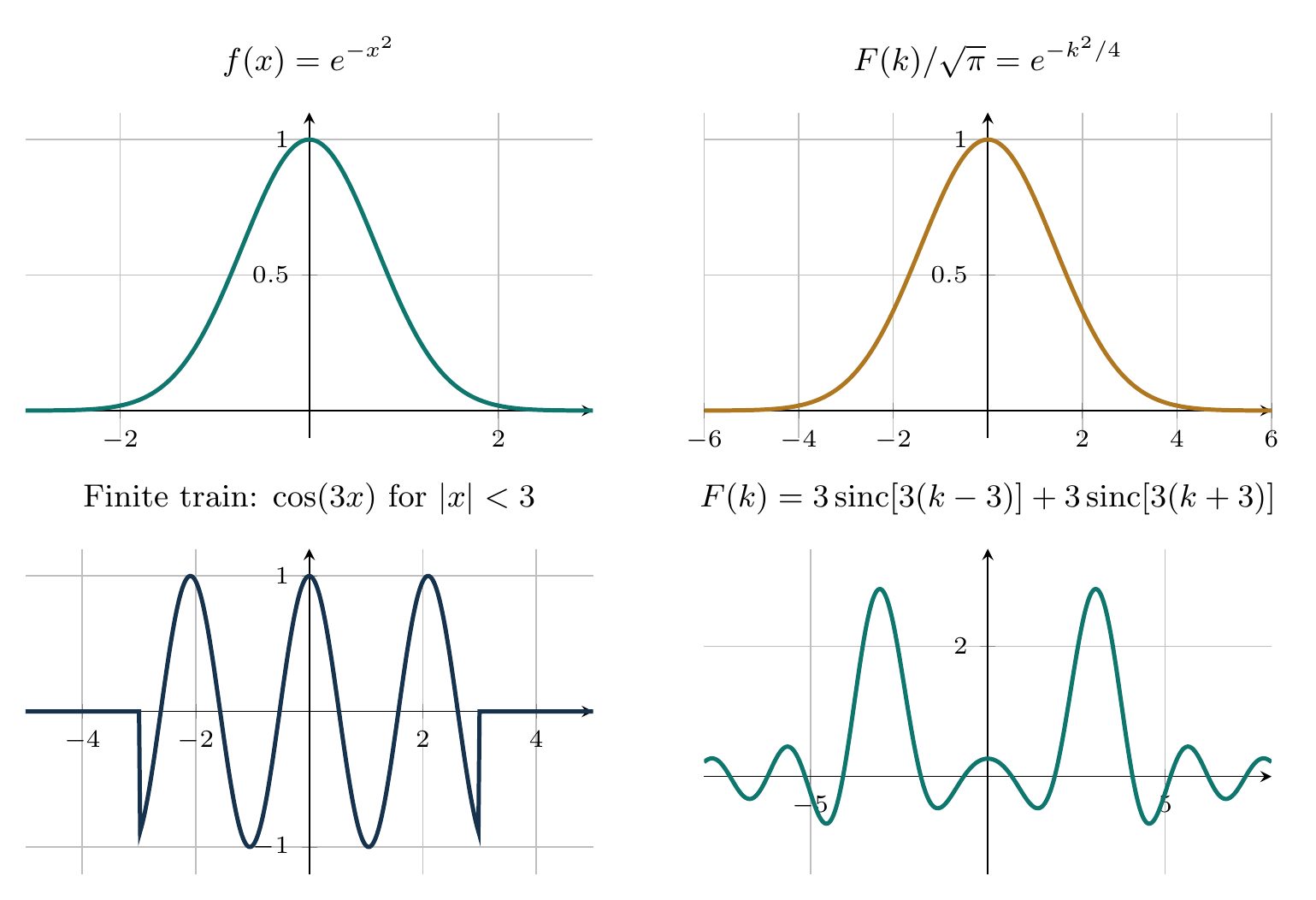
For $a>0$, let $f(x)=e^{-ax^2}$. Complete the square:
\[-ax^2-ikx =-a\left(x+\frac{ik}{2a}\right)^2-\frac{k^2}{4a}.\]The Gaussian integral is unchanged by the permitted contour displacement, so
\[\begin{aligned} F(k)&=e^{-k^2/(4a)} \int_{-\infty}^{\infty} e^{-a(x+ik/2a)^2}\,dx\\ &=\boxed{\sqrt{\frac\pi a}\,e^{-k^2/(4a)}}. \end{aligned}\]The dimensions are consistent: if $x$ is measured in metres, then $k$ is in $\mathrm{m}^{-1}$, $a$ is in $\mathrm{m}^{-2}$, and $F$ has the dimensions of $f$ times metres.
Finite pulse and finite wave train
For a rectangular pulse of width $L$,
\[f(x)=\begin{cases}1,&\lvert x\rvert<L/2,\\0,&\lvert x\rvert>L/2,\end{cases}\]direct integration gives
\[F(k)=\int_{-L/2}^{L/2}e^{-ikx}dx =\frac{2\sin(kL/2)}k =L\,\operatorname{sinc}\!\left(\frac{kL}{2}\right),\]where $\operatorname{sinc}u=\sin u/u$.
A finite cosine train is $f(x)=\cos(k_0x)$ for $\lvert x\rvert<L/2$ and zero otherwise. Using the two exponentials,
\[\boxed{ F(k)= \frac{\sin[(k-k_0)L/2]}{k-k_0} +\frac{\sin[(k+k_0)L/2]}{k+k_0}. }\]The apparent singularities at $k=\pm k_0$ are removable limits. Each sinc contribution by itself has first zeros $2\pi/L$ from its centre. When $k_0L\gg1$ the two contributions are well separated, so each peak has this approximate width; where they overlap, their sum need not vanish at those individual-sinc zeros.
Transform of derivatives
Assume $f$ and its required derivatives vanish at $\lvert x\rvert\to\infty$. Integration by parts gives
\[\begin{aligned} \mathcal F\{f^{\prime}(x)\} &=\left[f(x)e^{-ikx}\right]_{-\infty}^{\infty} +ik\int_{-\infty}^{\infty}f(x)e^{-ikx}dx\\ &=ikF(k). \end{aligned}\]Repeated integration gives
\[\boxed{\mathcal F\{f^{(n)}(x)\}=(ik)^nF(k).}\]If the boundary terms do not vanish, they must be retained.
Inverse transform
Insert the definition of $F(k)$ into the proposed inverse:
\[\begin{aligned} \frac1{2\pi}\int F(k)e^{ikx}dk &=\int f(x^{\prime})\left[ \frac1{2\pi}\int e^{ik(x-x^{\prime})}dk \right]dx^{\prime}\\ &=\int f(x^{\prime})\delta(x-x^{\prime})dx^{\prime}=f(x). \end{aligned}\]Thus the inverse formula follows directly from the Fourier representation of the delta distribution.
Convolution theorem
Define
\[(f\ast g)(x)=\int_{-\infty}^{\infty}f(u)g(x-u)\,du.\]Its transform is
\[\begin{aligned} \mathcal F\{f\ast g\} &=\int dx\,e^{-ikx}\int du\,f(u)g(x-u)\\ &=\int du\,f(u)e^{-iku} \int dy\,g(y)e^{-iky}\\ &=\boxed{F(k)G(k)}, \end{aligned}\]where $y=x-u$. Conversely,
\[\boxed{\mathcal F\{f(x)g(x)\}=\frac1{2\pi}(F*G)(k).}\]Solved Problems
1. Transform of a two-sided exponential
Find the Fourier transform of $f(x)=e^{-a\lvert x\rvert}$ for $a>0$. Splitting the integral at the origin removes the absolute value:
\[\begin{aligned} F(k) &=\int_{-\infty}^{0}e^{(a-ik)x}\,dx +\int_0^{\infty}e^{-(a+ik)x}\,dx\\ &=\frac1{a-ik}+\frac1{a+ik} =\boxed{\frac{2a}{a^2+k^2}}. \end{aligned}\]The assumption $a>0$ makes both boundary terms vanish. At $k=0$, $F(0)=2/a=\int f(x)dx$, which checks the sign and normalization. If $x$ is a length, then $a$ and $k$ have units $\mathrm{m}^{-1}$ and $F$ has units of $f$ times metres.
2. Convolution of two rectangular pulses
Let $p(x)=1$ for $\lvert x\rvert<a/2$ and zero otherwise. Determine $h=p\ast p$ and verify the convolution theorem directly.
The product $p(u)p(x-u)$ is nonzero where the intervals $(-a/2,a/2)$ and $(x-a/2,x+a/2)$ overlap. Their overlap has length $a-\lvert x\rvert$ when $\lvert x\rvert<a$ and no length otherwise, so
\[h(x)=\begin{cases} a-\lvert x\rvert,&\lvert x\rvert<a,\\ 0,&\lvert x\rvert>a. \end{cases}\]The pulse transform is
\[P(k)=\int_{-a/2}^{a/2}e^{-ikx}dx =\frac{2\sin(ka/2)}k.\]Because $h$ is even, its direct transform is
\[\begin{aligned} H(k)&=2\int_0^a(a-x)\cos(kx)\,dx\\ &=\frac{2[1-\cos(ka)]}{k^2} =\frac{4\sin^2(ka/2)}{k^2}=P^2(k). \end{aligned}\]The removable limit $H(0)=a^2$ equals $\int h(x)dx$. If $p$ is dimensionless, then $h$ has units of length and $H$ has units of length squared, as required by the two integrations.
3. A decaying Green function
Solve on the full line
\[-y^{\prime\prime}(x)+\alpha^2y(x)=\delta(x), \qquad y(x)\to0\quad\text{as}\quad\lvert x\rvert\to\infty,\]where $\alpha>0$. If $Y(k)=\mathcal{F}[y]$, the derivative rule gives $\mathcal{F}[y^{\prime\prime}]=-k^2Y$. Therefore
\[(k^2+\alpha^2)Y(k)=1, \qquad Y(k)=\frac1{k^2+\alpha^2}.\]The transform pair from Problem 1, with $a=\alpha$, now gives
\[\boxed{y(x)=\frac{e^{-\alpha\lvert x\rvert}}{2\alpha}.}\]Integrating the differential equation from $-\varepsilon$ to $+\varepsilon$ and taking $\varepsilon\to0$ yields the required jump
\[y^{\prime}(0^+)-y^{\prime}(0^-)=-1.\]The solution has $y^{\prime}(0^+)=-1/2$ and $y^{\prime}(0^-)=1/2$, so the sign is correct; it also satisfies the decay boundary conditions. Since $\delta(x)$ has units of inverse length and the operator has units of inverse length squared, $y$ has units of length.
Descriptive Questions
- Why are the Fourier transforms of infinite sine and cosine waves distributions rather than ordinary functions?
- How does integration by parts produce the transform-of-derivatives rule, and when do boundary terms survive?
- How does multiplication by a finite rectangular window broaden a monochromatic spectral line into sinc-shaped peaks?
- How do the direct and inverse Fourier-transform conventions determine the factor $1/(2\pi)$ in the product theorem?
Numerical Problems
-
Using the stated transform convention, find $F(4)$ for $f(x)=e^{-4x^2}$.
Final answer: $F(4)=\sqrt\pi/(2e)$.
-
A unit rectangular pulse has width $L=0.50\,\mathrm m$. Find $F(0)$ and the first nonzero spectral zeros.
Final answer: $F(0)=0.50\,\mathrm m$ and $k=\pm4\pi\,\mathrm{m}^{-1}$.
-
A finite cosine train has $L=2\,\mathrm m$ and $k_0=5\,\mathrm{m}^{-1}$. Evaluate the removable limit $F(k_0)$.
Final answer: $F(k_0)=[1+\sin(10)/10]\,\mathrm m$.
-
Find $\mathcal{F}[x e^{-x^2}]$ and evaluate it at $k=2$.
Final answer: $-ik\sqrt\pi e^{-k^2/4}/2$; at $k=2$ it is $-i\sqrt\pi/e$.
-
For $f(x)=3\delta(x-2)-\delta(x+1)$, find $F(k)$ and $F(\pi)$.
Final answer: $F(k)=3e^{-2ik}-e^{ik}$ and $F(\pi)=4$.
-
Convolve $e^{-x}H(x)$ with $e^{-2x}H(x)$ and evaluate the result at $x=\ln2$.
Final answer: $(e^{-x}-e^{-2x})H(x)$ and the value is $1/4$.
The transform pairs, theorem applications, all solved results, and every final answer are checked in the Maxima worksheet; every printed residual is zero.
References
- Fourier transform — Wikipedia
- NIST Digital Library of Mathematical Functions, §1.14: Integral Transforms
- MIT OpenCourseWare 18.103: Fourier Analysis lecture notes
- G. B. Arfken, H. J. Weber and F. E. Harris, Mathematical Methods for Physicists, 7th ed., chapter on integral transforms.


Discussion