22 Jul 2025

Quantum Perturbation Theory and Transitions

First- and second-order stationary perturbation theory, degenerate levels, the Stark effect, time-dependent amplitudes, transition probabilities, and Fermi's golden rule.

mj-18 perturbation-theory stark-effect transition-probability fermi-golden-rule

Let

\[H=H_0+\lambda V, \qquad H_0\lvert n^{(0)}\rangle=E_n^{(0)}\lvert n^{(0)}\rangle,\]

and expand

\[E_n=E_n^{(0)}+\lambda E_n^{(1)}+\lambda^2E_n^{(2)}+\cdots,\] \[\lvert n\rangle=\lvert n^{(0)}\rangle+\lambda\lvert n^{(1)}\rangle +\lambda^2\lvert n^{(2)}\rangle+\cdots.\]

Choose intermediate normalization, $\langle n^{(0)}\mid n\rangle=1$, so $\langle n^{(0)}\mid n^{(j)}\rangle=0$ for $j\ge1$.

Nondegenerate time-independent theory

Insert the expansions into $H\lvert n\rangle=E_n\lvert n\rangle$ and compare first powers of $\lambda$:

\[(H_0-E_n^{(0)})\lvert n^{(1)}\rangle =(E_n^{(1)}-V)\lvert n^{(0)}\rangle.\]

Projection with $\langle n^{(0)}\rvert$ makes the left side zero and gives

\[\boxed{E_n^{(1)}=V_{nn},} \qquad V_{mn}=\langle m^{(0)}\rvert V\lvert n^{(0)}\rangle.\]

For $m\ne n$,

\[(E_m^{(0)}-E_n^{(0)}) \langle m^{(0)}\mid n^{(1)}\rangle=-V_{mn},\]

so

\[\boxed{ \lvert n^{(1)}\rangle =\sum_{m\ne n} \frac{V_{mn}}{E_n^{(0)}-E_m^{(0)}}\lvert m^{(0)}\rangle. }\]

At second order,

\[(H_0-E_n^{(0)})\lvert n^{(2)}\rangle =(E_n^{(1)}-V)\lvert n^{(1)}\rangle +E_n^{(2)}\lvert n^{(0)}\rangle.\]

Projection with $\langle n^{(0)}\rvert$ and intermediate normalization give

\[E_n^{(2)}=\langle n^{(0)}\rvert V\lvert n^{(1)}\rangle.\]

Substituting the first-order ket yields

\[\boxed{ E_n^{(2)} =\sum_{m\ne n} \frac{\lvert V_{mn}\rvert^2}{E_n^{(0)}-E_m^{(0)}}. }\]

These formulas require the perturbation matrix elements to be small compared with the relevant nonzero energy separations.

Degenerate case

Suppose $g$ orthonormal states $\lvert a\rangle$ share the unperturbed energy $E_d^{(0)}$. The zeroth-order ket inside this subspace is $\lvert\psi^{(0)}\rangle=\sum_{b=1}^gc_b\lvert b\rangle$. Projecting the first-order equation onto $\langle a\rvert$ gives

\[\sum_{b=1}^g(V_{ab}-E^{(1)}\delta_{ab})c_b=0.\]

A nonzero coefficient vector exists only if

\[\boxed{\det(V_{ab}-E^{(1)}\delta_{ab})=0.}\]

Thus the correct zeroth-order combinations are the eigenvectors of $V$ restricted to the degenerate subspace. Coupling to states outside that subspace then supplies the second-order correction through the nonzero energy denominators.

Linear Stark effect in hydrogen

Take a uniform electric field $\mathcal E\hat{\mathbf z}$. With scalar potential $\Phi=-\mathcal Ez$, the electron perturbation energy is

\[V=(-e)\Phi=e\mathcal Ez.\]

Since

\[\cos\theta\,Y_l^m =A_{lm}Y_{l+1}^m+B_{lm}Y_{l-1}^m,\]

the angular integral imposes the electric-dipole selection rules

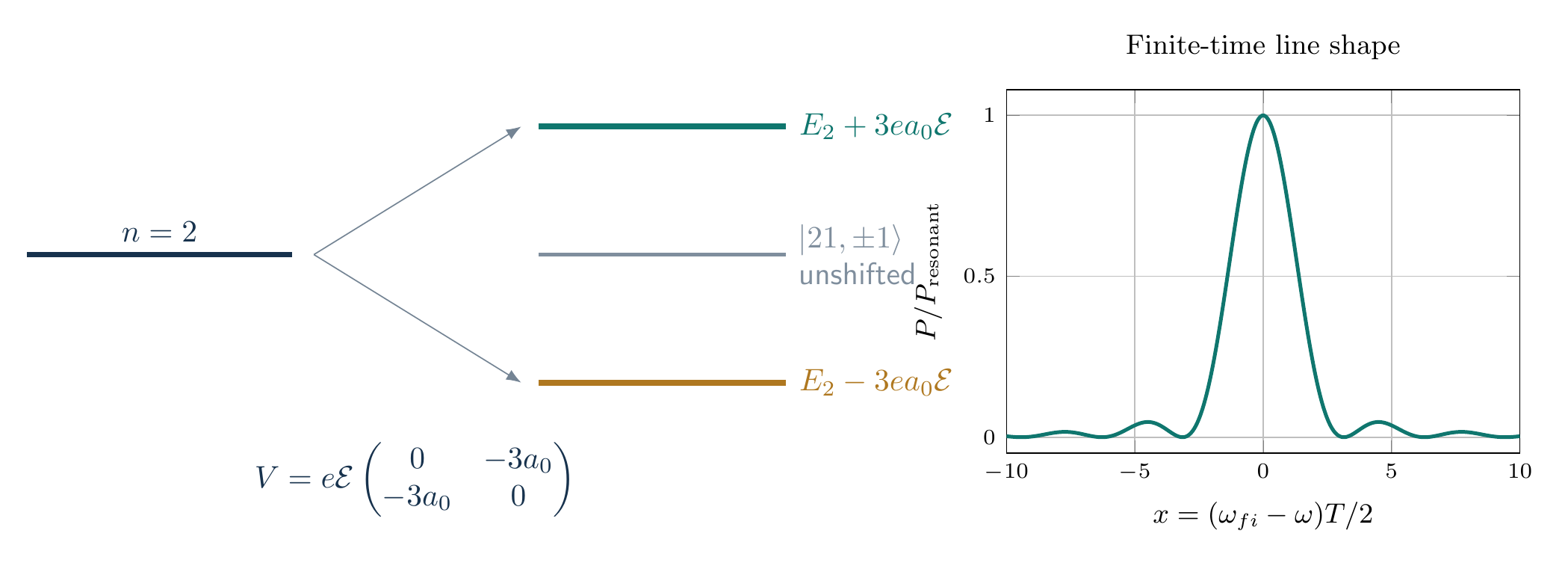
\[\boxed{\Delta l=\pm1,\qquad \Delta m=0}\]

for a field along $z$. In the $n=2$ manifold, only $\lvert200\rangle$ and $\lvert210\rangle$ mix. With $x=r/a_0$,

\[\psi_{200}=\frac{(2-x)e^{-x/2}}{4\sqrt{2\pi}\,a_0^{3/2}}, \qquad \psi_{210}=\frac{x e^{-x/2}\cos\theta} {4\sqrt{2\pi}\,a_0^{3/2}}.\]

Parity makes the two diagonal matrix elements zero. The off-diagonal element is

\[\begin{aligned} \langle200\rvert z\lvert210\rangle &=\frac1{32\pi a_0^3} \int_0^\infty r^2dr\,(2-x)xe^{-x}r \int\cos^2\theta\,d\Omega\\ &=\frac1{32\pi a_0^3} \left[a_0^4\int_0^\infty x^4(2-x)e^{-x}dx\right] \left(\frac{4\pi}{3}\right)\\ &=\frac{a_0}{24}[2(4!)-5!] =-3a_0. \end{aligned}\]

Therefore, in the ordered basis $(\lvert200\rangle,\lvert210\rangle)$,

\[V=e\mathcal E \begin{pmatrix}0&-3a_0\\-3a_0&0\end{pmatrix}.\]

Its normalized eigenvectors and shifts are

\[\lvert\pm\rangle=\frac{\lvert200\rangle\mp\lvert210\rangle}{\sqrt2}, \qquad \boxed{E_\pm^{(1)}=\pm3ea_0\mathcal E.}\]

The $\lvert21,\pm1\rangle$ states have zero first-order shift because $\Delta m=0$ forbids their coupling to the $2s$ state.

Time-dependent perturbation theory

Let $H(t)=H_0+V(t)$ and expand an exact state as

\[\lvert\Psi(t)\rangle=\sum_n c_n(t)e^{-iE_nt/\hbar}\lvert n\rangle.\]

Insert this in $i\hbar\partial_t\lvert\Psi\rangle=H\lvert\Psi\rangle$. The $H_0$ terms cancel, leaving

\[i\hbar\dot c_f(t) =\sum_nV_{fn}(t)e^{i\omega_{fn}t}c_n(t), \qquad \omega_{fn}=\frac{E_f-E_n}{\hbar}.\]

If the system begins in $\lvert i\rangle$, first order replaces $c_n(t)$ on the right by $\delta_{ni}$:

\[\boxed{ c_f^{(1)}(t) =-\frac{i}{\hbar}\int_0^t V_{fi}(t')e^{i\omega_{fi}t'}dt', \qquad f\ne i. }\]

The transition probability to this order is

\[\boxed{P_{i\to f}(t)=\lvert c_f^{(1)}(t)\rvert^2.}\]

Constant perturbation

For $V_{fi}(t)=V_{fi}$ during $0<t<T$,

\[\begin{aligned} c_f^{(1)}(T) &=-\frac{iV_{fi}}{\hbar} \frac{e^{i\omega_{fi}T}-1}{i\omega_{fi}}\\ &=-\frac{2iV_{fi}}{\hbar} e^{i\omega_{fi}T/2} \frac{\sin(\omega_{fi}T/2)}{\omega_{fi}}. \end{aligned}\]

Hence

\[\boxed{ P_{i\to f}(T) =\frac{4\lvert V_{fi}\rvert^2}{\hbar^2} \frac{\sin^2(\omega_{fi}T/2)}{\omega_{fi}^2}. }\]

At $\omega_{fi}=0$, the limiting probability is $\lvert V_{fi}\rvert^2T^2/\hbar^2$.

Harmonic perturbation and Fermi’s golden rule

Write a real harmonic perturbation as

\[V(t)=We^{-i\omega t}+W^\dagger e^{i\omega t}.\]

The absorption part of the first-order amplitude is

\[c_{f,\rm abs}^{(1)}(T) =-\frac{iW_{fi}}{\hbar} e^{i(\omega_{fi}-\omega)T/2} \frac{2\sin[(\omega_{fi}-\omega)T/2]} {\omega_{fi}-\omega}.\]

It is sharply peaked at the energy-selection condition

\[\boxed{E_f-E_i=\hbar\omega.}\]

The conjugate term produces the stimulated-emission amplitude

\[c_{f,\rm em}^{(1)}(T) =-\frac{i(W^\dagger)_{fi}}{\hbar} e^{i(\omega_{fi}+\omega)T/2} \frac{2\sin[(\omega_{fi}+\omega)T/2]} {\omega_{fi}+\omega},\]

which is resonant when

\[\boxed{E_f-E_i=-\hbar\omega.}\]

For final states forming a continuum with density $\rho(E_f)$, use

\[\lim_{T\to\infty} \frac1T\frac{4\sin^2[(E_f-E_i-\hbar\omega)T/(2\hbar)]} {(E_f-E_i-\hbar\omega)^2} =\frac{2\pi}{\hbar}\delta(E_f-E_i-\hbar\omega).\]

Integration over final energies gives Fermi’s golden rule,

\[\boxed{ \Gamma_{i\to f} =\frac{2\pi}{\hbar}\lvert W_{fi}\rvert^2\rho(E_f) \bigg\rvert_{E_f=E_i+\hbar\omega}. }\]

If the perturbation is written $V_0\cos\omega t$, then $W=V_0/2$ for the absorption component. Any additional selection rules follow from a vanishing matrix element. For an electric dipole, $\Delta l=\pm1$. Polarization along $z$ selects $\Delta m=0$; transverse linear polarization is a superposition of $\Delta m=+1$ and $-1$, while a fixed circular helicity selects one of these two signs. An arbitrary polarization can contain all three spherical components $\Delta m=0,\pm1$.

The \(n=2\) hydrogen subspace splits by \(\pm3ea_0\mathcal E\); a finite interaction time produces the exact squared-sinc energy profile.

The stationary perturbation expansion, Stark integrals and eigenvectors, constant-pulse amplitude, and parity-forbidden diagonal element are checked in the Maxima worksheet; every printed residual is zero.