

30 Jul 2025
Quantum Scattering Theory
Cross sections, wave packets, Green functions, partial waves, Coulomb and Born scattering, the optical theorem, phase shifts, scattering length, and effective range.
For a localized potential $V(\mathbf r)$ and energy $E=\hbar^2k^2/(2\mu)$, choose the incident wave along $z$. The stationary scattering state has the large-distance form
\[\boxed{ \psi(\mathbf r)\underset{r\to\infty}{\sim} e^{ikz}+f(\theta,\phi)\frac{e^{ikr}}r. }\]The first term is the incident plane wave; the second is an outgoing spherical wave. This boundary condition excludes incoming waves from infinity.
Differential and total cross sections
The probability current is
\[\mathbf j=\frac{\hbar}{2\mu i} (\psi^*\nabla\psi-\psi\nabla\psi^*).\]For $e^{ikz}$, $j_{\rm in}=\hbar k/\mu$. For the outgoing term, keeping the leading power at large $r$,
\[j_{\mathrm{sc},r} =\frac{\hbar k}{\mu r^2}\lvert f(\theta,\phi)\rvert^2.\]The rate crossing $r^2d\Omega$ divided by incident flux is therefore
\[\boxed{\frac{d\sigma}{d\Omega}=\lvert f(\theta,\phi)\rvert^2,} \qquad \boxed{\sigma_{\rm tot}=\int\lvert f\rvert^2d\Omega.}\]$f$ has dimensions of length and a cross section has dimensions of area.
Scattering of a wave packet
A physical incident state is a packet,
\[\Psi(\mathbf r,t)=\frac{1}{(2\pi)^{3/2}}\int a(\mathbf k) \psi_{\mathbf k}^{(+)}(\mathbf r) e^{-i\hbar k^2t/(2\mu)}d^3k,\]where the scattering states use the plane-wave convention $\langle\psi_{\mathbf k}^{(+)}\mid\psi_{\mathbf k^{\prime}}^{(+)}\rangle =(2\pi)^3\delta^3(\mathbf k-\mathbf k^{\prime})$. Thus $a(\mathbf k)$ is concentrated near $\mathbf k_0$ and $\int\lvert a(\mathbf k)\rvert^2d^3k=1$. Before collision, the incoming part is localized; after collision, the outgoing packet separates spatially. The stationary cross section is recovered when the packet is narrow enough that $f$ and the incident speed vary negligibly across its momentum width.
Green function and scattering amplitude
The stationary Schrödinger equation is
\[(E-H_0)\psi=V\psi, \qquad H_0=-\frac{\hbar^2}{2\mu}\nabla^2.\]Define the outgoing Green function by
\[(E-H_0)G^{(+)}(\mathbf r-\mathbf r^{\prime}) =\delta^3(\mathbf r-\mathbf r^{\prime}).\]Since
\[(\nabla^2+k^2)\frac{e^{ikR}}R=-4\pi\delta^3(\mathbf R),\]its normalization is
\[\boxed{ G^{(+)}(\mathbf R) =-\frac{\mu}{2\pi\hbar^2}\frac{e^{ikR}}R. }\]Adding a free incident solution gives the Lippmann-Schwinger equation
\[\psi(\mathbf r)=e^{i\mathbf k\cdot\mathbf r} -\frac{\mu}{2\pi\hbar^2} \int\frac{e^{ik\lvert\mathbf r-\mathbf r^{\prime}\rvert}} {\lvert\mathbf r-\mathbf r^{\prime}\rvert} V(\mathbf r^{\prime})\psi(\mathbf r^{\prime})d^3r^{\prime}.\]For $r$ much larger than the range of the potential,
\[\lvert\mathbf r-\mathbf r^{\prime}\rvert\simeq r-\hat{\mathbf r}\cdot\mathbf r^{\prime}, \qquad \frac1{\lvert\mathbf r-\mathbf r^{\prime}\rvert}\simeq\frac1r.\]Comparison with the asymptotic definition identifies $\mathbf k^{\prime}=k\hat{\mathbf r}$ and
\[\boxed{ f(\mathbf k^{\prime},\mathbf k) =-\frac{\mu}{2\pi\hbar^2} \int e^{-i\mathbf k^{\prime}\cdot\mathbf r^{\prime}} V(\mathbf r^{\prime})\psi(\mathbf r^{\prime})d^3r^{\prime}. }\]This formula is exact; its unknown scattering state remains inside the integral.
Born approximation
When the scattered wave is small inside the interaction region, replace $\psi(\mathbf r^{\prime})$ by the incident plane wave. The first Born amplitude is
\[\boxed{ f_B(\mathbf q) =-\frac{\mu}{2\pi\hbar^2} \int e^{-i\mathbf q\cdot\mathbf r}V(\mathbf r)d^3r, \qquad \mathbf q=\mathbf k^{\prime}-\mathbf k. }\]Elastic scattering has $\lvert\mathbf k^{\prime}\rvert=\lvert\mathbf k\rvert=k$, so
\[q^2=\lvert\mathbf k^{\prime}-\mathbf k\rvert^2 =2k^2(1-\cos\theta)=4k^2\sin^2\frac\theta2.\]The approximation requires the potential-induced wave to remain small; it is generally reliable for weak potentials or sufficiently large incident energy.
Scattering in a Coulomb field
Let $V(r)=\kappa_C/r$. Because the Coulomb field is long-ranged, introduce $e^{-\eta r}$ and take $\eta\to0^+$ after transforming:
\[\begin{aligned} \int e^{-i\mathbf q\cdot\mathbf r} \frac{e^{-\eta r}}r\,d^3r &=\frac{4\pi}{q}\int_0^\infty e^{-\eta r}\sin(qr)dr\\ &=\frac{4\pi}{q^2+\eta^2} \longrightarrow\frac{4\pi}{q^2}. \end{aligned}\]Thus the screened Born limit gives
\[f_C(\theta) =-\frac{2\mu\kappa_C}{\hbar^2q^2} =-\frac{\mu\kappa_C} {2\hbar^2k^2\sin^2(\theta/2)}.\]Using $E=\hbar^2k^2/(2\mu)$,
\[\boxed{ \frac{d\sigma_C}{d\Omega} =\frac{\kappa_C^2}{16E^2\sin^4(\theta/2)}. }\]This is the Rutherford angular dependence. The unscreened Coulomb potential also produces a long-range logarithmic phase, so the short-range asymptotic phase conventions used below must not be applied to it without modification.
Partial-wave analysis and phase shifts
For a central short-range potential, expand the incident wave as
\[e^{ikz}=\sum_{l=0}^{\infty} i^l(2l+1)j_l(kr)P_l(\cos\theta).\]Since
\[j_l(kr)\sim\frac1{kr} \sin\left(kr-\frac{l\pi}{2}\right),\]the incident plane wave contains, in each $l$ channel, equal incoming and outgoing radial flux. Outside the potential range, the radial solution obeys $u_l^{\prime\prime}+[k^2-l(l+1)/r^2]u_l=0$ and may be written
\[\boxed{ u_l(r)\sim A_l \sin\left(kr-\frac{l\pi}{2}+\delta_l\right). }\]$\delta_l$ is the phase shift. Writing the sine as two exponentials shows that the outgoing-to-incoming ratio changes from its free value by
\[S_l=e^{2i\delta_l}.\]Elastic flux conservation gives $\lvert S_l\rvert=1$, so $\delta_l$ is real. Keep the incoming coefficient equal to the plane-wave value and replace only the outgoing coefficient by $S_l$. Subtracting the free outgoing part gives
\[f(\theta)=\frac1{2ik}\sum_{l=0}^{\infty} (2l+1)(S_l-1)P_l(\cos\theta).\]Since $(e^{2i\delta_l}-1)/(2i)=e^{i\delta_l}\sin\delta_l$,
\[\boxed{ f(\theta)=\frac1k\sum_{l=0}^{\infty} (2l+1)e^{i\delta_l}\sin\delta_lP_l(\cos\theta). }\]Legendre orthogonality,
\[\int P_l(\cos\theta)P_{l^{\prime}}(\cos\theta)d\Omega =\frac{4\pi}{2l+1}\delta_{ll^{\prime}},\]then gives
\[\boxed{ \sigma_{\rm tot}=\frac{4\pi}{k^2} \sum_{l=0}^{\infty}(2l+1)\sin^2\delta_l. }\]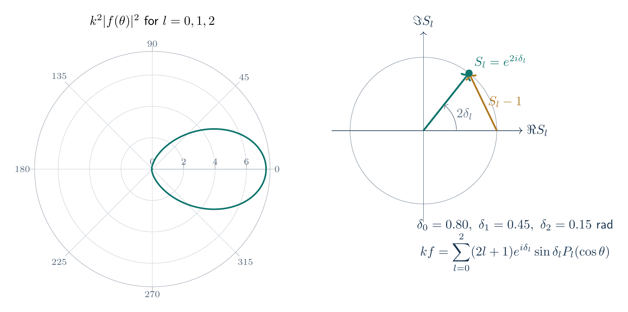
Optical theorem
At $\theta=0$, $P_l(1)=1$, so
\[\operatorname{Im}f(0) =\frac1k\sum_l(2l+1) \operatorname{Im}[e^{i\delta_l}\sin\delta_l] =\frac1k\sum_l(2l+1)\sin^2\delta_l.\]Comparison with the total cross section gives
\[\boxed{ \sigma_{\rm tot}=\frac{4\pi}{k}\operatorname{Im}f(0). }\]The relation follows from probability conservation, even though it connects the total cross section to the strictly forward amplitude.
Scattering length and effective range
At sufficiently small $k$, a finite-range potential is dominated by $l=0$. Its amplitude is
\[f_0(k)=\frac{e^{2i\delta_0}-1}{2ik} =\boxed{\frac1{k\cot\delta_0-ik}}.\]At zero energy and outside the potential range, the radial equation is $u_0^{\prime\prime}=0$. Normalize its solution as
\[u_0(r)\longrightarrow1-\frac ra.\]The intercept $a$ is the scattering length. Matching this limit to $\sin(kr+\delta_0)$ gives
\[\lim_{k\to0}k\cot\delta_0=-\frac1a, \qquad f_0(0)=-a, \qquad \boxed{\sigma_{k\to0}=4\pi a^2.}\]For a short-range potential, the next even power defines the effective range:
\[\boxed{ k\cot\delta_0=-\frac1a+\frac12r_ek^2+O(k^4). }\]If the zero-energy solution is normalized as above, comparison of the finite- and zero-energy radial equations gives Bethe’s integral form
\[\boxed{ r_e=2\int_0^\infty \left[\left(1-\frac ra\right)^2-u_0^2(r)\right]dr. }\]The integral terminates effectively outside the interaction range because the two terms then coincide. Substitution into $f_0(k)$ describes the leading finite-energy correction to scattering-length behavior.
Solved Problems
1. First Born scattering from a Gaussian potential
Let
\[V(r)=V_0e^{-r^2/a^2}.\]Choose the $z$ axis along $\mathbf q$. The three-dimensional Fourier integral may be evaluated as a product of Cartesian Gaussian integrals:
\[\begin{aligned} \int e^{-i\mathbf q\cdot\mathbf r}e^{-r^2/a^2}d^3r &=\prod_{j=x,y,z}\int_{-\infty}^{\infty} e^{-x_j^2/a^2-iq_jx_j}dx_j\\ &=(\sqrt\pi a)^3 \exp\left(-\frac{a^2q^2}{4}\right). \end{aligned}\]Substitution into the Born formula gives
\[\boxed{ f_B(q)=-\frac{\mu V_0\sqrt\pi a^3}{2\hbar^2} e^{-a^2q^2/4}, \qquad q=2k\sin\frac\theta2.}\]Therefore
\[\boxed{ \frac{d\sigma_B}{d\Omega} =\frac{\pi\mu^2V_0^2a^6}{4\hbar^4} \exp\left(-\frac{a^2q^2}{2}\right).}\]$\mu V_0a^3/\hbar^2$ has units of length, so the cross section has units of area. The forward value is largest, the angular width decreases as $ka$ increases, and the result vanishes continuously as $V_0\to0$.
2. Partial waves and the optical theorem
Suppose only $l=0$ and $l=1$ contribute, with $\delta_0=30^\circ$, $\delta_1=10^\circ$, and $k=2.00\,\mathrm{nm^{-1}}$. The total cross section is
\[\begin{aligned} \sigma_{\rm tot} &=\frac{4\pi}{k^2} [\sin^2\delta_0+3\sin^2\delta_1]\\ &=\pi[0.25+3(0.0301537)]\,\mathrm{nm^2}\\ &=\boxed{1.06959\,\mathrm{nm^2}}. \end{aligned}\]The imaginary part of the forward amplitude is
\[\operatorname{Im}f(0) =\frac1k[\sin^2\delta_0+3\sin^2\delta_1] =0.170231\,\mathrm{nm}.\]Consequently
\[\frac{4\pi}{k}\operatorname{Im}f(0) =1.06959\,\mathrm{nm^2}=\sigma_{\rm tot},\]which verifies the optical theorem with consistent length and area units. If both phase shifts tend to zero, the cross section tends to zero.
3. Effective-range correction at low energy
Take scattering length $a=5.00\,\mathrm{fm}$, effective range $r_e=1.50\,\mathrm{fm}$, and $k=0.100\,\mathrm{fm^{-1}}$. To order $k^2$,
\[k\cot\delta_0 =-\frac1a+\frac12r_ek^2 =-0.200+0.00750 =-0.19250\,\mathrm{fm^{-1}}.\]Thus
\[f_0(k)=\frac1{-0.19250-i(0.100)}\,\mathrm{fm},\]and the $s$-wave cross section is
\[\begin{aligned} \sigma_0 &=4\pi\lvert f_0\rvert^2 =\frac{4\pi}{(0.19250)^2+(0.100)^2}\,\mathrm{fm^2}\\ &=\boxed{267.050\,\mathrm{fm^2}}. \end{aligned}\]The denominator has units $\mathrm{fm^{-2}}$, so the result has units of area. As $k\to0$, the effective-range term and $ik$ vanish and the formula reduces to $4\pi a^2=314.159\,\mathrm{fm^2}$.
Descriptive Questions
- Explain why a localized incident wave packet is physically required and how the stationary differential cross section emerges in its narrow-momentum limit.
- Derive the outgoing Green function and the Lippmann-Schwinger equation, keeping the normalization, sign, and outgoing boundary condition explicit.
- Obtain the first Born amplitude, state its regime of validity, and explain why a screened limit is needed before transforming the Coulomb potential.
- Derive the partial-wave amplitude, total cross section, optical theorem, and effective-range expansion for a short-range central potential.
Numerical Problems
- If $f(\theta)=0.400\cos\theta\,\mathrm{nm}$, calculate $d\sigma/d\Omega$ at $\theta=60^\circ$ and the total cross section.
- A normalized momentum-space packet has $a(\mathbf k)=C\exp[-\lvert\mathbf k-\mathbf k_0\rvert^2/(4s^2)]$ with $s=0.200\,\mathrm{nm^{-1}}$. Find $C$ from $\int\lvert a\rvert^2d^3k=1$.
- For elastic scattering with $k=5.00\,\mathrm{nm^{-1}}$ and $\theta=60^\circ$, find the momentum-transfer magnitude $q$.
- Evaluate the Rutherford differential cross section for $\kappa_C=1.44\,\mathrm{eV\,nm}$, $E=1.00\,\mathrm{keV}$, and $\theta=30^\circ$.
Final answers: 1. $0.0400\,\mathrm{nm^2\,sr^{-1}}$ and $0.670206\,\mathrm{nm^2}$; 2. $C=(2\pi s^2)^{-3/4}=2.817\,\mathrm{nm^{3/2}}$; 3. $q=5.00\,\mathrm{nm^{-1}}$; 4. $2.88815\times10^{-5}\,\mathrm{nm^2\,sr^{-1}}$.
The core derivations and all problem answers are checked in the original Maxima worksheet and the problems worksheet; every printed residual is zero.
References
- Scattering theory.
- J. J. Sakurai and J. Napolitano, Modern Quantum Mechanics, 3rd ed., Chapter 6, “Scattering Theory.”
- D. J. Griffiths and D. F. Schroeter, Introduction to Quantum Mechanics, 3rd ed., Chapter 11, “Scattering.”
- J. R. Taylor, Scattering Theory: The Quantum Theory of Nonrelativistic Collisions, Dover ed., Chapters 1–3.


Discussion