

06 May 2025
Retarded Potentials and Liénard-Wiechert Fields
Causal electromagnetic potentials and the exact electric and magnetic fields of a point charge in uniform or arbitrary motion.
In the Lorenz gauge,
\[\nabla\cdot\mathbf A+\frac{1}{c^2}\frac{\partial\phi}{\partial t}=0,\]Maxwell’s equations reduce to wave equations,
\[\left(\nabla^2-\frac{1}{c^2}\frac{\partial^2}{\partial t^2}\right)\phi =-\frac{\rho}{\epsilon_0}, \qquad \left(\nabla^2-\frac{1}{c^2}\frac{\partial^2}{\partial t^2}\right)\mathbf A =-\mu_0\mathbf J.\]The retarded Green function is
\[G_{\rm ret}(\mathbf r,t;\mathbf r^{\prime},t^{\prime}) =\frac{\delta\!\left(t-t^{\prime}-\lvert\mathbf r-\mathbf r^{\prime}\rvert/c\right)} {4\pi\lvert\mathbf r-\mathbf r^{\prime}\rvert}.\]It vanishes unless a signal emitted at $(\mathbf r^{\prime},t^{\prime})$ can reach $(\mathbf r,t)$ at speed $c$. Convolution with the sources gives
\[\boxed{ \phi(\mathbf r,t)=\frac{1}{4\pi\epsilon_0} \int\frac{\rho(\mathbf r^{\prime},t-R/c)}{R}\,d^3r^{\prime}, }\] \[\boxed{ \mathbf A(\mathbf r,t)=\frac{\mu_0}{4\pi} \int\frac{\mathbf J(\mathbf r^{\prime},t-R/c)}{R}\,d^3r^{\prime}, } \qquad R=\lvert\mathbf r-\mathbf r^{\prime}\rvert.\]These are the retarded potentials. Their SI units are volts and tesla-metres, respectively.
For time-independent sources the retardation disappears from the integrands:
\[\phi(\mathbf r)=\frac{1}{4\pi\epsilon_0} \int\frac{\rho(\mathbf r^{\prime})}{R}\,d^3r^{\prime}, \qquad \mathbf A(\mathbf r)=\frac{\mu_0}{4\pi} \int\frac{\mathbf J(\mathbf r^{\prime})}{R}\,d^3r^{\prime}.\]Thus the causal solution has the correct electrostatic and magnetostatic limits. In particular, a stationary point charge gives $\phi=q/(4\pi\epsilon_0R)$, $\mathbf E=q\mathbf n/(4\pi\epsilon_0R^2)$, and $\mathbf B=0$.
Point charge and retarded geometry
Let a charge $q$ follow $\mathbf r_q(t)$. Its density and current are
\[\rho(\mathbf r,t)=q\,\delta^3[\mathbf r-\mathbf r_q(t)], \qquad \mathbf J(\mathbf r,t)=q\mathbf v(t)\, \delta^3[\mathbf r-\mathbf r_q(t)].\]For a fixed observation event $(\mathbf r,t)$, define
\[t_r=t-\frac{R(t_r)}{c},\qquad \mathbf R=\mathbf r-\mathbf r_q(t_r),\qquad R=\lvert\mathbf R\rvert,\qquad \mathbf n=\frac{\mathbf R}{R},\] \[\boldsymbol\beta=\frac{\mathbf v(t_r)}{c}, \qquad \kappa=1-\mathbf n\cdot\boldsymbol\beta.\]To make the schematic trajectory equation-generated, use the dimensionless path parameter $\tau=(t^{\prime}-t_r)/(t-t_r)$ and diagram coordinates
\[x_d(\tau)=-2.2+3.2\tau, \qquad y_d(\tau)=-0.8\tau^2(1-\tau), \qquad 0\le\tau\le1.\]Thus the two source events are the plotted endpoints at $\tau=0$ and $1$; the field derivation itself retains an arbitrary $\mathbf r_q(t)$.
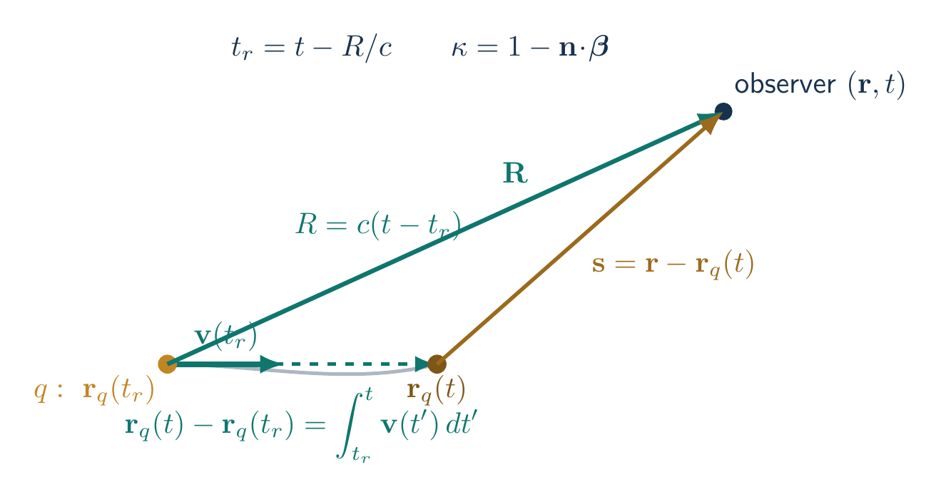
When the delta function is integrated over source time, its argument $g(t^{\prime})=t-t^{\prime}-R(t^{\prime})/c$ contributes the Jacobian
\[\left\lvert\frac{dg}{dt^{\prime}}\right\rvert_{t_r} =\left\lvert-1+\frac{\mathbf n\cdot\mathbf v}{c}\right\rvert_{t_r} =\kappa.\]Therefore the Liénard-Wiechert potentials are
\[\boxed{ \phi(\mathbf r,t)=\left[\frac{q}{4\pi\epsilon_0\kappa R}\right]_{t_r}, \qquad \mathbf A(\mathbf r,t)=\left[\frac{\mu_0q\mathbf v}{4\pi\kappa R}\right]_{t_r} =\frac{\boldsymbol\beta}{c}\phi. }\]Differentiating retarded quantities
The implicit definition of $t_r$ must be differentiated before computing $\mathbf E=-\nabla\phi-\partial_t\mathbf A$. At fixed $\mathbf r$,
\[\frac{dt_r}{dt} =1-\frac{1}{c}\frac{dR}{dt_r}\frac{dt_r}{dt}, \qquad \frac{dR}{dt_r}=-\mathbf n\cdot\mathbf v,\]so
\[\boxed{\frac{dt_r}{dt}=\frac{1}{\kappa}}.\]At fixed $t$, take a spatial gradient of $t-t_r-R(t_r)/c=0$:
\[-\nabla t_r-\frac{1}{c} \left(\mathbf n+\frac{dR}{dt_r}\nabla t_r\right)=0,\]which gives
\[\boxed{\nabla t_r=-\frac{\mathbf n}{c\kappa}}.\]For any source quantity $Q$ whose observation-point dependence occurs only through $t_r$,
\[\frac{\partial Q(t_r)}{\partial t}=\frac{\dot Q}{\kappa}, \qquad \nabla Q(t_r)=-\frac{\mathbf n\dot Q}{c\kappa}.\]The remaining geometric derivatives follow before any field differentiation:
\[\frac{\partial R}{\partial t} =\frac{dR}{dt_r}\frac{dt_r}{dt} =-\frac{c\,\mathbf n\cdot\boldsymbol\beta}{\kappa}, \qquad \nabla R=\mathbf n+\frac{dR}{dt_r}\nabla t_r =\frac{\mathbf n}{\kappa},\] \[\frac{\partial\mathbf n}{\partial t} =\frac{c[(\mathbf n\cdot\boldsymbol\beta)\mathbf n-\boldsymbol\beta]} {\kappa R}, \qquad \frac{d\kappa}{dt_r} =\frac{c[\beta^2-(\mathbf n\cdot\boldsymbol\beta)^2]}R -\mathbf n\cdot\dot{\boldsymbol\beta}.\]The spatial dependence of $\mathbf n$ must also be retained. In components,
\[\frac{\partial n_i}{\partial r_j} =\frac1R\left[\delta_{ij} +\frac{(\beta_i-n_i)n_j}{\kappa}\right].\]Consequently, with $b=\mathbf n\cdot\boldsymbol\beta$,
\[\boxed{ \nabla\kappa =-\frac{\boldsymbol\beta}{R} -\frac{\beta^2-b}{\kappa R}\mathbf n +\frac{\mathbf n\cdot\dot{\boldsymbol\beta}}{c\kappa}\mathbf n. }\]Put $C=q/(4\pi\epsilon_0)$. Since $\partial_t\kappa=\dot\kappa/\kappa$, direct differentiation of $\phi=C/(\kappa R)$ and $\mathbf A=\boldsymbol\beta\phi/c$ gives
\[\nabla\phi=-C\left[ \frac{\nabla\kappa}{\kappa^2R} +\frac{\mathbf n}{\kappa^2R^2}\right],\] \[\frac{\partial\mathbf A}{\partial t} =\frac Cc\left[ \frac{\dot{\boldsymbol\beta}}{\kappa^2R} +\boldsymbol\beta\left( \frac{cb}{\kappa^2R^2}-\frac{\dot\kappa}{\kappa^3R} \right)\right].\]Substitute the displayed formulas for $\nabla\kappa$ and $\dot\kappa$ into $\mathbf E=-\nabla\phi-\partial_t\mathbf A$. Separating inverse powers of $R$ gives
\[\begin{aligned} \frac{\mathbf E}{C} ={}&\frac1{R^2}\left[ \frac{\mathbf n-(1+b)\boldsymbol\beta}{\kappa^2} -\frac{(\beta^2-b)\mathbf n}{\kappa^3} +\frac{(\beta^2-b^2)\boldsymbol\beta}{\kappa^3} \right]\\ &+\frac1{c\kappa^3R}\left[ (\mathbf n\cdot\dot{\boldsymbol\beta}) (\mathbf n-\boldsymbol\beta) -\kappa\dot{\boldsymbol\beta}\right]. \end{aligned}\]Using $\kappa=1-b$, the $R^{-2}$ coefficients reduce as
\[\kappa-(\beta^2-b)=1-\beta^2,\] \[-(1+b)\kappa+(\beta^2-b^2)=-(1-\beta^2).\]The vector triple-product identity gives
\[(\mathbf n\cdot\dot{\boldsymbol\beta}) (\mathbf n-\boldsymbol\beta)-\kappa\dot{\boldsymbol\beta} =\mathbf n\times[(\mathbf n-\boldsymbol\beta) \times\dot{\boldsymbol\beta}].\]Therefore
\[\boxed{ \mathbf E(\mathbf r,t)=\frac{q}{4\pi\epsilon_0} \left[ \frac{(1-\beta^2)(\mathbf n-\boldsymbol\beta)}{\kappa^3R^2} +\frac{\mathbf n\times[(\mathbf n-\boldsymbol\beta) \times\dot{\boldsymbol\beta}]}{c\kappa^3R} \right]_{t_r}, }\]For the magnetic field,
\[\nabla\times\boldsymbol\beta =\nabla t_r\times\dot{\boldsymbol\beta} =-\frac{\mathbf n\times\dot{\boldsymbol\beta}}{c\kappa},\]so
\[\mathbf B=\nabla\times\mathbf A =\frac1c\left(\nabla\phi\times\boldsymbol\beta -\frac{\phi}{c\kappa}\mathbf n\times\dot{\boldsymbol\beta}\right).\]Inserting $\nabla\phi$ and collecting its $R^{-2}$ and $R^{-1}$ terms gives
\[\boxed{\mathbf B(\mathbf r,t)=\frac{1}{c}\mathbf n\times\mathbf E.}\]Here $\dot{\boldsymbol\beta}=d\boldsymbol\beta/dt_r$. The first term is the velocity field, proportional to $R^{-2}$; the second is the acceleration field, proportional to $R^{-1}$. Dimensional checking gives $q/(\epsilon_0R^2)$ for the first term and $q\dot\beta/(\epsilon_0cR)$ for the second, both in volts per metre.
Uniform rectilinear motion
For $\mathbf v=$ constant, $\dot{\boldsymbol\beta}=0$. Express the field in terms of the vector from the present charge position to the observer,
\[\mathbf s=\mathbf r-\mathbf r_q(t),\qquad \mathbf s=\mathbf s_\parallel+\mathbf s_\perp,\]where the subscripts are relative to $\mathbf v$. For uniform motion, $\mathbf r_q(t)=\mathbf r_q(t_r)+\mathbf v(t-t_r)$ and $c(t-t_r)=R$, so
\[\mathbf s=\mathbf R-\boldsymbol\beta R =R(\mathbf n-\boldsymbol\beta).\]Its parallel and perpendicular components obey
\[s_\parallel=R(\mathbf n\cdot\hat{\mathbf v}-\beta), \qquad s_\perp=R\sqrt{1-(\mathbf n\cdot\hat{\mathbf v})^2}.\]A direct expansion then gives
\[s_\parallel^2+(1-\beta^2)s_\perp^2 =R^2(1-\mathbf n\cdot\boldsymbol\beta)^2 =R^2\kappa^2.\]Since $\mathbf n-\boldsymbol\beta=\mathbf s/R$, the velocity field becomes
\[\boxed{ \mathbf E=\frac{q}{4\pi\epsilon_0} \frac{(1-\beta^2)\mathbf s} {\left[s_\parallel^2+(1-\beta^2)s_\perp^2\right]^{3/2}}, \qquad \mathbf B=\frac{1}{c^2}\mathbf v\times\mathbf E. }\]On the line of motion, $\mathbf s_\perp=0$ and $E=q/(4\pi\epsilon_0\gamma^2s^2)$. In the transverse plane, $s_\parallel=0$ and $E=\gamma q/(4\pi\epsilon_0s^2)$. Thus increasing $\gamma=(1-\beta^2)^{-1/2}$ suppresses the longitudinal field and compresses the field into transverse directions. The arbitrary-motion formula above reduces continuously to this result when the acceleration is set to zero.
Solved Problems
1. Retarded event for transverse observation
A charge $q=1.00\ \mathrm{nC}$ moves uniformly as $\mathbf r_q(t)=0.800ct\,\hat{\mathbf x}$. At observation time $t=0$, find the retarded time and scalar potential at $\mathbf r=0.300\,\hat{\mathbf y}\ \mathrm m$.
The retardation condition is
\[0=t_r+\frac1c\sqrt{(0.800ct_r)^2+(0.300\ \mathrm m)^2}.\]The physical root must satisfy $t_r<0$. Squaring and retaining that root,
\[c^2t_r^2=0.800^2c^2t_r^2+(0.300\ \mathrm m)^2,\] \[t_r=-\frac{\gamma(0.300\ \mathrm m)}c, \qquad \gamma=\frac1{\sqrt{1-0.800^2}}=\frac53,\]so $t_r=-1.668\ \mathrm{ns}$ and $R=-ct_r=0.500\ \mathrm m$. At the retarded event,
\[n_x=\frac{-0.800ct_r}{R}=0.800, \qquad \kappa=1-n_x\beta=1-0.800^2=0.360.\]Consequently,
\[\phi=\frac{q}{4\pi\epsilon_0\kappa R} =\frac{(8.98755\times10^9)(1.00\times10^{-9})} {(0.360)(0.500)} =49.93\ \mathrm V.\]The units are $({\rm V\,m})/{\rm m}={\rm V}$. The enhancement relative to $q/(4\pi\epsilon_0R)$ is the Jacobian factor $1/\kappa$; it is not an instantaneous interaction.
2. Electric flux of a uniformly moving charge
Show that the anisotropic uniform-motion field still has total flux $q/\epsilon_0$ through a sphere of radius $s$ centred on the present charge position.
If $\theta$ is measured from $\mathbf v$, the field is radial from the present position and has magnitude
\[E(s,\theta)=\frac{q}{4\pi\epsilon_0s^2} \frac{1-\beta^2}{(1-\beta^2\sin^2\theta)^{3/2}}.\]Therefore
\[\Phi_E=2\pi s^2\int_0^\pi E(s,\theta)\sin\theta\,d\theta.\]With $u=\cos\theta$ and $a=1-\beta^2$,
\[\begin{aligned} \Phi_E &=\frac{q}{2\epsilon_0}(1-\beta^2) \int_{-1}^{1}\frac{du}{(a+\beta^2u^2)^{3/2}}\\ &=\frac{q}{2\epsilon_0}(1-\beta^2) \left[\frac{u}{a\sqrt{a+\beta^2u^2}}\right]_{-1}^{1}\\ &=\frac{q}{2\epsilon_0}(1-\beta^2)\frac{2}{1-\beta^2} =\boxed{\frac q{\epsilon_0}}. \end{aligned}\]The angular compression redistributes flux but does not change its total. The radius cancels, as required by Gauss’s law, and the $\beta\to0$ limit is the Coulomb result.
Descriptive Questions
- Derive the factor $\kappa=1-\mathbf n\cdot\boldsymbol\beta$ when the point-charge source is integrated over retarded time, and explain its causal meaning.
- Starting from the implicit retardation condition, obtain $\partial t_r/\partial t$ and $\nabla t_r$, keeping clear which variables are held fixed.
- Separate the Liénard-Wiechert electric field into its $R^{-2}$ and $R^{-1}$ parts and identify the assumptions behind each limiting form.
- Derive the present-position field of a charge in uniform rectilinear motion and explain its longitudinal suppression and transverse enhancement.
Numerical Problems
- A stationary charge of $4.00\ \mathrm{nC}$ is observed at $R=0.500\ \mathrm m$. Find its retarded scalar potential and electric-field magnitude.
- At equal present separation from a uniformly moving charge, compare the longitudinal and transverse fields for $\beta=0.900$ with the Coulomb magnitude $E_C$.
- A charge $2.00\ \mathrm{nC}$ moves with $\beta=0.600$. At present separation $s=0.400\ \mathrm m$, the separation vector makes $60.0^\circ$ with the velocity. Find $E$ and $B$.
- In the nonrelativistic transverse direction, at what distance are the velocity and acceleration fields equal in magnitude if $a=3.00\times10^{16}\ \mathrm{m\,s^{-2}}$?
- A charge $1.00\ \mathrm{\mu C}$ has nonrelativistic acceleration $1.00\times10^{12}\ \mathrm{m\,s^{-2}}$. Find $E_{\rm rad}$ and $B_{\rm rad}$ at $R=100\ \mathrm m$ and $\theta=30.0^\circ$.
Answers: 1. $\phi=71.90\ \mathrm V$, $E=143.8\ \mathrm{V\,m^{-1}}$; 2. $\gamma=2.294$, $E_\parallel=0.1900E_C$, $E_\perp=2.294E_C$, and $E_\perp/E_\parallel=12.07$; 3. $E=115.3\ \mathrm{V\,m^{-1}}$ along $\mathbf s$, $B=1.998\times10^{-7}\ \mathrm T$ along $\mathbf v\times\mathbf s$; 4. $R=c^2/a=2.996\ \mathrm m$; 5. $E_{\rm rad}=5.000\times10^{-4}\ \mathrm{V\,m^{-1}}$, $B_{\rm rad}=1.668\times10^{-12}\ \mathrm T$.
The retarded-time identities, flux integral, uniform-motion reductions, and all printed numerical answers are checked in the Maxima worksheet; every printed residual is zero.
References
- Liénard-Wiechert potential
- David J. Griffiths, Introduction to Electrodynamics, 4th ed., Chapter 10, “Potentials and Fields.”
- John D. Jackson, Classical Electrodynamics, 3rd ed., Chapter 14, “Radiation by Moving Charges.”
- The Feynman Lectures on Physics, Vol. II, Chapter 26, “Lorentz Transformations of the Fields”


Discussion