

29 May 2026
Dispersion and Absorption in Solids
Lorentz oscillators, resonance line shapes, normal and anomalous dispersion, causality, Kramers–Kronig relations, oscillator strengths, and Cauchy and Sellmeier formulas.
Dispersion is the variation of a material’s optical response with frequency, while absorption is the irreversible transfer of electromagnetic energy to the solid. The two phenomena are not independent. A resonance that absorbs energy also produces a rapid change in the real refractive index, and causality connects the real and imaginary parts of every linear response function through the Kramers–Kronig relations.
The convention used here is $e^{-i\omega t}$. A passive material consequently has $\varepsilon’’(\omega)>0$ and extinction coefficient $\kappa>0$ for positive frequency.
Bound-charge equation of motion
Consider an electron of charge $-e$ whose displacement $\mathbf x$ from equilibrium is opposed by a harmonic restoring force. Let $m$ be the effective mass, $\omega_0$ the natural angular frequency and $\gamma$ the damping rate. Its equation of motion is
\[m\ddot{\mathbf x}+m\gamma\dot{\mathbf x} +m\omega_0^2\mathbf x=-e\mathbf E(t).\]For $\mathbf E(t)=\mathbf E_0e^{-i\omega t}$ and $\mathbf x(t)=\mathbf x_0e^{-i\omega t}$,
\[m(\omega_0^2-\omega^2-i\gamma\omega)\mathbf x_0 =-e\mathbf E_0,\]so
\[\mathbf x_0=-\frac{e\mathbf E_0/m} {\omega_0^2-\omega^2-i\gamma\omega}.\]The induced dipole moment of one oscillator is $\mathbf p=-e\mathbf x$. For $N$ identical oscillators per unit volume,
\[\mathbf P=N\mathbf p =\frac{Ne^2/m}{\omega_0^2-\omega^2-i\gamma\omega} \mathbf E.\]Since $\mathbf P=\varepsilon_0\chi\mathbf E$,
\[\boxed{ \chi(\omega)= \frac{\Omega^2} {\omega_0^2-\omega^2-i\gamma\omega}, \qquad \Omega^2=\frac{Ne^2}{\varepsilon_0m} }.\]The parameter $\Omega$ measures oscillator spectral weight; it is not the resonance frequency $\omega_0$. If other, remote processes contribute a slowly varying background $\varepsilon_\infty$,
\[\boxed{ \varepsilon(\omega)=\varepsilon_\infty+ \frac{\Omega^2} {\omega_0^2-\omega^2-i\gamma\omega} }.\]An equivalent form uses the static dielectric increment
\[\Delta\varepsilon=\frac{\Omega^2}{\omega_0^2},\]giving
\[\varepsilon(\omega)=\varepsilon_\infty+ \frac{\Delta\varepsilon\,\omega_0^2} {\omega_0^2-\omega^2-i\gamma\omega}.\]The Drude response is the $\omega_0=0$ limit, for which there is no restoring force and the resonance is centred at zero frequency.
Real and imaginary parts
Let
\[a=\omega_0^2-\omega^2, \qquad b=\gamma\omega.\]Using $(a-ib)^{-1}=(a+ib)/(a^2+b^2)$ gives
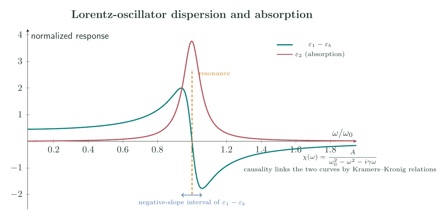
\[\boxed{ \varepsilon'(\omega)=\varepsilon_\infty+ \frac{\Omega^2(\omega_0^2-\omega^2)} {(\omega_0^2-\omega^2)^2+\gamma^2\omega^2} },\] \[\boxed{ \varepsilon''(\omega)= \frac{\Omega^2\gamma\omega} {(\omega_0^2-\omega^2)^2+\gamma^2\omega^2} }.\]The imaginary part is positive for $\omega>0$ and represents absorption. At resonance,
\[\varepsilon'(\omega_0)=\varepsilon_\infty, \qquad \varepsilon''(\omega_0)=\frac{\Omega^2}{\gamma\omega_0} =\frac{\Delta\varepsilon\,\omega_0}{\gamma}.\]Weak damping produces a tall, narrow absorption band; strong damping produces a lower, broader band.
Near a weakly damped resonance, write $\omega=\omega_0+\delta$ with $\lvert\delta\rvert\ll\omega_0$. Then
\[\omega_0^2-\omega^2\simeq-2\omega_0\delta, \qquad \gamma\omega\simeq\gamma\omega_0,\]and
\[\varepsilon''(\omega) \simeq \frac{\Omega^2\gamma/\omega_0} {4\delta^2+\gamma^2}.\]This local Lorentzian has half-width at half-maximum $\gamma/2$ and full width at half-maximum $\gamma$. Away from the weak-damping limit, the exact maximum of $\varepsilon’’$ is slightly shifted from $\omega_0$, and the full expression must be used.
Absorption coefficient
For a nonmagnetic solid,
\[(n+i\kappa)^2=\varepsilon'+i\varepsilon'',\]so
\[\varepsilon'=n^2-\kappa^2, \qquad \varepsilon''=2n\kappa.\]The exact intensity absorption coefficient is
\[\boxed{ \alpha(\omega)=\frac{2\omega\kappa(\omega)}{c} }.\]In a weakly absorbing spectral region, $\kappa\ll n$. Then $\varepsilon’\simeq n^2$ and
\[\kappa\simeq\frac{\varepsilon''}{2n}.\]Therefore
\[\boxed{ \alpha(\omega)\simeq \frac{\omega\varepsilon''(\omega)}{n(\omega)c} \qquad(\kappa\ll n) }.\]The cycle-averaged absorbed power density is
\[\langle p\rangle =\frac12\omega\varepsilon_0\varepsilon'' \lvert\mathbf E_0\rvert^2.\]Thus a positive $\varepsilon’’$ is both the cause of spatial attenuation and the coefficient governing local electromagnetic heating.
Multiple resonances and oscillator strengths
A real solid contains many infrared-active lattice modes and electronic transitions. A classical multi-oscillator representation is
\[\boxed{ \varepsilon(\omega)=\varepsilon_\infty+ \sum_j\frac{S_j} {\omega_j^2-\omega^2-i\gamma_j\omega} }.\]Here $S_j$ has dimensions of angular frequency squared. In a quantum-mechanical oscillator-strength notation for $N$ atoms or formula units per unit volume,
\[\boxed{ \varepsilon(\omega)=1+ \frac{Ne^2}{\varepsilon_0m_e} \sum_j \frac{f_j}{\omega_j^2-\omega^2-i\gamma_j\omega} }.\]The dimensionless $f_j$ measures the strength of transition $j$. For a complete set of transitions from one initial state, the Thomas–Reiche–Kuhn sum rule fixes the total oscillator strength. With an appropriate count of active electrons,
\[\sum_j f_j=Z.\]The corresponding dielectric spectral-weight relation is
\[\boxed{ \int_0^\infty \omega\varepsilon''(\omega)\,d\omega =\frac{\pi}{2} \sum_j S_j }.\]For the optical conductivity, $\sigma_1=\varepsilon_0\omega\varepsilon’’$, so this becomes the optical $f$-sum rule
\[\int_0^\infty\sigma_1(\omega)\,d\omega =\frac{\pi}{2}\varepsilon_0\sum_jS_j.\]Line broadening redistributes absorption in frequency but does not change the total spectral weight of an oscillator.
Normal and anomalous dispersion
In a transparent interval sufficiently far from resonance, damping can be neglected:
\[\varepsilon'(\omega) \simeq\varepsilon_\infty+ \frac{\Omega^2}{\omega_0^2-\omega^2}.\]Below resonance,
\[\frac{d\varepsilon'}{d\omega} =\frac{2\Omega^2\omega} {(\omega_0^2-\omega^2)^2}>0.\]Since $n\simeq\sqrt{\varepsilon’}$, this normally gives $dn/d\omega>0$: the refractive index increases with frequency and decreases with vacuum wavelength. This is normal dispersion.
Within and immediately around an absorption band, damping cannot be omitted. The real part changes rapidly from above to below its background value and can contain a range with
\[\frac{dn}{d\omega}<0.\]This is anomalous dispersion. It does not violate causality; it occurs precisely because absorption and dispersion are linked. In a transparent, weakly dispersive region the group velocity is
\[\boxed{ v_g=\left(\frac{dk}{d\omega}\right)^{-1} =\frac{c}{n+\omega\,dn/d\omega} }.\]Inside a strongly absorbing band, $k$ is complex and a pulse is reshaped. The expression above may then give a value that is not the velocity of energy or information, so energy velocity and signal-front propagation must be treated using the full causal response.
Causality and Kramers–Kronig relations
In a linear causal medium, the polarization at time $t$ depends only on earlier fields:
\[P(t)=\varepsilon_0\int_0^\infty \chi(\tau)E(t-\tau)\,d\tau.\]The frequency-domain susceptibility is
\[\chi(\omega)=\int_0^\infty \chi(\tau)e^{i\omega\tau}\,d\tau.\]Because the integral contains no negative times, $\chi(\omega)$ is analytic in the upper half of the complex $\omega$ plane. Cauchy’s theorem then relates its boundary values on the real axis. For a response that tends to zero at high frequency,
\[\boxed{ \chi'(\omega)=\frac{1}{\pi}\mathcal P \int_{-\infty}^{\infty} \frac{\chi''(\Omega)}{\Omega-\omega}\,d\Omega },\] \[\boxed{ \chi''(\omega)=-\frac{1}{\pi}\mathcal P \int_{-\infty}^{\infty} \frac{\chi'(\Omega)}{\Omega-\omega}\,d\Omega }.\]Here $\mathcal P$ denotes the Cauchy principal value. Since a real time-domain response implies $\chi’(-\omega)=\chi’(\omega)$ and $\chi’’(-\omega)=-\chi’’(\omega)$, the positive-frequency forms are
\[\boxed{ \chi'(\omega)=\frac{2}{\pi}\mathcal P \int_0^\infty \frac{\Omega\chi''(\Omega)}{\Omega^2-\omega^2}\,d\Omega },\] \[\boxed{ \chi''(\omega)=-\frac{2\omega}{\pi}\mathcal P \int_0^\infty \frac{\chi'(\Omega)}{\Omega^2-\omega^2}\,d\Omega }.\]For a dielectric function that approaches $\varepsilon_\infty$ over the extrapolated high-frequency range, apply these relations to $\varepsilon-\varepsilon_\infty$. In particular,
\[\boxed{ \varepsilon'(0)-\varepsilon_\infty =\frac{2}{\pi}\int_0^\infty \frac{\varepsilon''(\Omega)}{\Omega}\,d\Omega }.\]Every absorption band therefore contributes to the static real permittivity. Conversely, a measured absorption spectrum constrains dispersion at all frequencies. Practical Kramers–Kronig analysis requires extrapolation outside the experimental window, so the low- and high-frequency extrapolations are part of the physical model.
Cauchy dispersion formula
In a transparent range lying well below all relevant electronic resonances, neglect damping and expand
\[\frac{1}{\omega_j^2-\omega^2} =\frac{1}{\omega_j^2} \left[1+\frac{\omega^2}{\omega_j^2} +\frac{\omega^4}{\omega_j^4}+\cdots\right].\]The dielectric function then has an even-power expansion in frequency. Since $\omega=2\pi c/\lambda$, taking the square root gives the empirical Cauchy formula
\[\boxed{ n(\lambda)=A+\frac{B}{\lambda^2} +\frac{C}{\lambda^4}+\cdots }.\]The numerical values and dimensions of $B,C,\ldots$ depend on the unit used for $\lambda$. The formula is valid only in a transparent interval remote from absorption bands. It does not represent the absorption coefficient and should not be extrapolated through a resonance.
Sellmeier dispersion formula
Set damping to zero and express each Lorentz term through its resonance wavelength $\lambda_j=2\pi c/\omega_j$. If $B_j=S_j/\omega_j^2$, then
\[\frac{S_j}{\omega_j^2-\omega^2} =\frac{B_j\lambda^2}{\lambda^2-\lambda_j^2}.\]For a nonmagnetic transparent solid, $n^2\simeq\varepsilon’$, so the Sellmeier formula is
\[\boxed{ n^2(\lambda)=1+ \sum_j\frac{B_j\lambda^2} {\lambda^2-C_j}, \qquad C_j=\lambda_j^2 }.\]Some fitted forms absorb a constant background into the leading term rather than writing it as unity. Sellmeier coefficients represent effective ultraviolet and infrared resonances and give a more physically structured transparent-region interpolation than a short Cauchy series. Because damping is absent, the standard real-coefficient formula must not be used to calculate absorption inside a band.
For wavelengths large compared with all $\sqrt{C_j}$ included in an ultraviolet-only model,
\[\frac{B_j\lambda^2}{\lambda^2-C_j} =B_j\left(1+\frac{C_j}{\lambda^2} +\frac{C_j^2}{\lambda^4}+\cdots\right).\]Expansion of the square root then reduces Sellmeier dispersion to a Cauchy series over the same restricted interval.
Worked Lorentz-oscillator calculation
Take
\[\varepsilon_\infty=2.25, \qquad \Delta\varepsilon=3.00, \qquad \gamma=0.10\omega_0.\]At $\omega=0.80\omega_0$, substitution into the exact expressions gives
\[\varepsilon'=10.19, \qquad \varepsilon''=1.765,\]and hence
\[n=3.204, \qquad \kappa=0.275.\]At resonance,
\[\varepsilon'=2.25, \qquad \varepsilon''=30.0,\]so the extinction is very strong. At $\omega=1.20\omega_0$,
\[\varepsilon'=-4.096, \qquad \varepsilon''=1.731,\]giving
\[n=0.419, \qquad \kappa=2.067.\]The reversal of the oscillator contribution to $\varepsilon’$ across the absorption band is the characteristic dispersive signature of a Lorentz resonance.
Worked Sellmeier and Cauchy calculation
Consider a one-resonance transparent-region model with wavelength measured in $\mu\mathrm m$:
\[n^2(\lambda)=1+ \frac{1.20\lambda^2}{\lambda^2-(0.150)^2}.\]At $\lambda=0.500\ \mu\mathrm m$,
\[n=1.5227,\]while at $\lambda=0.700\ \mu\mathrm m$,
\[n=1.5026.\]The index decreases as wavelength increases, which is normal dispersion. Expanding the model through order $\lambda^{-2}$ gives
\[n(\lambda)\simeq1.4832 +\frac{0.00910}{\lambda^2},\]with $\lambda$ still in $\mu\mathrm m$. This approximation gives $n=1.5197$ at $0.500\ \mu\mathrm m$ and $n=1.5018$ at $0.700\ \mu\mathrm m$. The closer agreement at the longer wavelength is expected because the expansion parameter is $\lambda_0^2/\lambda^2$.
Preparation questions
- Derive the complex Lorentz-oscillator susceptibility from the damped equation of motion.
- Obtain the real and imaginary parts of the dielectric function and discuss their signs on the two sides of resonance.
- Derive the weak-damping Lorentzian form near resonance and identify its full width at half-maximum.
- Relate the extinction coefficient and absorption coefficient to $\varepsilon’’$ in both exact and weak-absorption forms.
- Explain the oscillator-strength representation and derive the relation between dielectric and conductivity spectral weights.
- Distinguish normal and anomalous dispersion, and explain why anomalous dispersion is associated with absorption.
- Derive the group velocity in a transparent dispersive medium and explain why it requires care inside an absorbing band.
- State and interpret the positive-frequency Kramers–Kronig relations for the $e^{-i\omega t}$ convention.
- Derive the static-permittivity sum rule from the first Kramers–Kronig relation.
- Derive the Cauchy formula as a far-from-resonance expansion and state its domain of validity.
- Obtain the Sellmeier formula from a set of undamped Lorentz oscillators.
- Given Lorentz parameters or Sellmeier coefficients, calculate $\varepsilon’$, $\varepsilon’’$, $n$, $\kappa$, $\alpha$ or $dn/d\lambda$ at a specified frequency.


Discussion