

08 Jun 2026
Dynamic Dielectric Response and Alternating Fields
Complex permittivity, oscillator and relaxation models, frequency-dependent polarization, dielectric loss, absorption, and Kramers–Kronig relations.
An alternating electric field probes both the magnitude and the response time of polarization. Electronic clouds, ionic sublattices, permanent dipoles, and interfacial charges follow the field on different time scales. Their delayed response makes the permittivity complex and frequency dependent.
Throughout this post the physical field is the real part of
\[\mathbf E(t)=\mathbf E_0e^{-i\omega t}.\]With this convention a passive dielectric is written
\[\epsilon_r(\omega)=\epsilon_r'(\omega)+i\epsilon_r''(\omega), \qquad \epsilon_r''(\omega)\ge0\]for $\omega>0$. Texts using $e^{+i\omega t}$ attach the opposite sign to the imaginary part. All permittivities are relative unless an absolute permittivity is explicitly denoted by $\varepsilon=\epsilon_0\epsilon_r$.
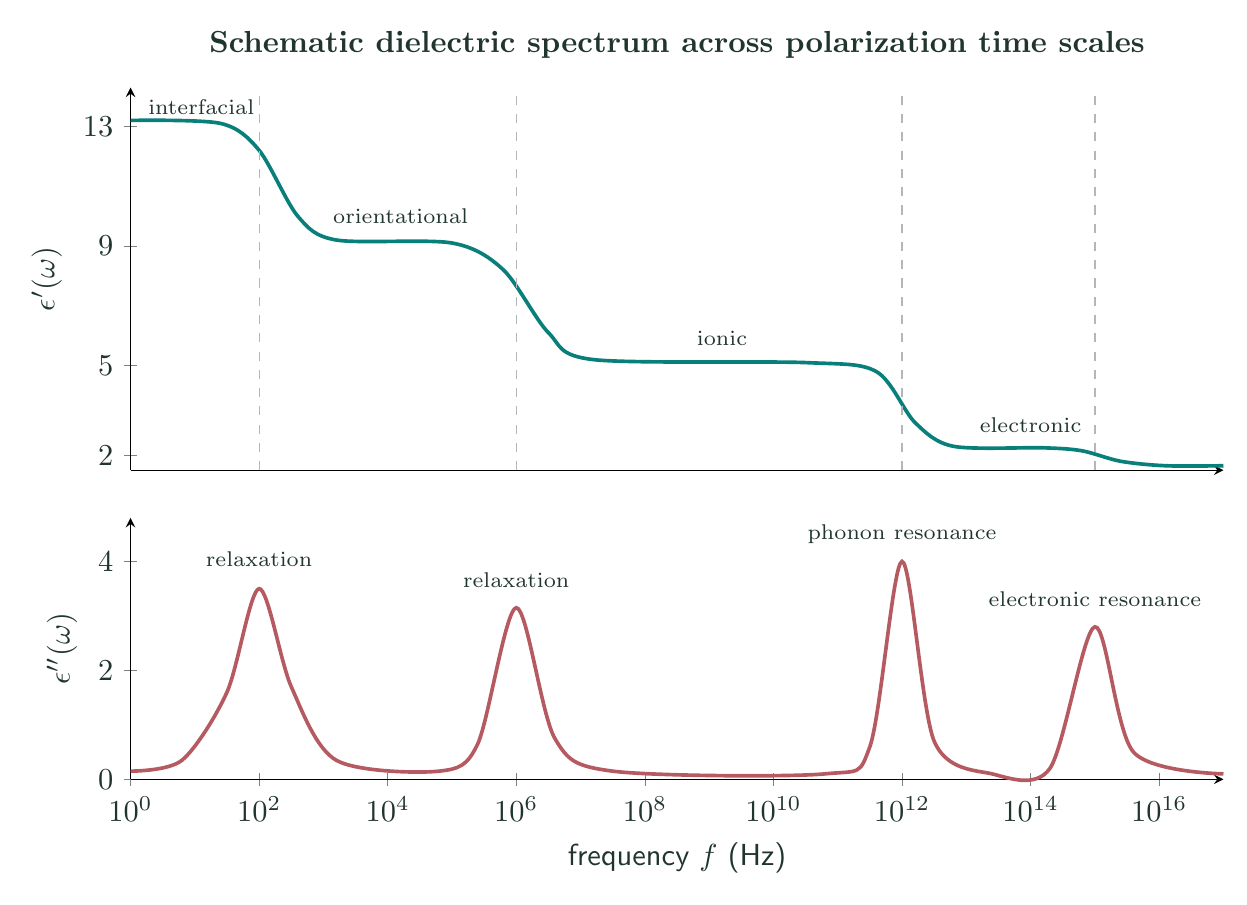
Linear response in the time and frequency domains
In a linear causal medium, the polarization at time $t$ can depend only on fields at earlier times:
\[P_i(t)=\epsilon_0\sum_j\int_0^\infty \chi_{ij}(\tau)E_j(t-\tau)\,d\tau.\]For a monochromatic field,
\[P_i(\omega)=\epsilon_0\sum_j\chi_{ij}(\omega)E_j(\omega),\]where
\[\chi_{ij}(\omega)=\int_0^\infty \chi_{ij}(\tau)e^{i\omega\tau}\,d\tau.\]For an isotropic material,
\[\mathbf D(\omega)=\epsilon_0\epsilon_r(\omega)\mathbf E(\omega), \qquad \epsilon_r(\omega)=1+\chi(\omega).\]The real part describes the component of polarization in phase with the field. The positive imaginary part describes the component lagging the field and is responsible for irreversible energy absorption.
Dielectric loss and power dissipation
The polarization-current phasor is
\[\mathbf J_P=-i\omega\mathbf P =-i\omega\epsilon_0\chi\mathbf E.\]For phasors with the $e^{-i\omega t}$ convention, the cycle average of $\mathbf E(t)\cdot\mathbf J_P(t)$ is
\[\langle p\rangle =\frac12\operatorname{Re}(\mathbf E_0\boldsymbol\cdot\mathbf J_{P0}^*) =\frac12\omega\epsilon_0\chi''|\mathbf E_0|^2.\]Since the vacuum contribution is real, $\chi’’=\epsilon_r’’$, and
\[\boxed{ \langle p\rangle =\frac12\omega\epsilon_0\epsilon_r''(\omega)|\mathbf E_0|^2 }.\]The dielectric loss tangent is
\[\boxed{\tan\delta=\frac{\epsilon_r''}{\epsilon_r'}}.\]If an ohmic conductivity $\sigma_{\mathrm{dc}}$ is present,
\[\mathbf J_{\mathrm{tot}} =\sigma_{\mathrm{dc}}\mathbf E-i\omega\epsilon_0\epsilon_{r,b}\mathbf E =-i\omega\epsilon_0 \left(\epsilon_{r,b}+i\frac{\sigma_{\mathrm{dc}}}{\epsilon_0\omega}\right)\mathbf E.\]Thus conduction may be represented by
\[\epsilon_{r,\mathrm{eff}}'' =\epsilon_{r,b}''+\frac{\sigma_{\mathrm{dc}}}{\epsilon_0\omega}.\]The $1/\omega$ contribution is not a bound-charge polarization resonance; it is free-charge dissipation included in an effective complex permittivity.
Lorentz-oscillator response
Electronic and ionic polarization are naturally modelled as damped oscillators. Let a normal coordinate $x$ have effective mass $m$, effective charge $q$, natural frequency $\omega_0$, and damping rate $\gamma$:
\[m\ddot x+m\gamma\dot x+m\omega_0^2x=qE(t).\]For $x(t)=x_0e^{-i\omega t}$,
\[x_0=\frac{qE_0/m}{\omega_0^2-\omega^2-i\gamma\omega}.\]If there are $N$ such oscillators per unit volume and $p=qx$, then
\[P=Nqx\]and
\[\boxed{ \chi(\omega)= \frac{Nq^2/(\epsilon_0m)} {\omega_0^2-\omega^2-i\gamma\omega} }.\]Define the oscillator strength parameter
\[\Omega_p^2=\frac{Nq^2}{\epsilon_0m}\]and write $a=\omega_0^2-\omega^2$, $b=\gamma\omega$. Since
\[\frac1{a-ib}=\frac{a+ib}{a^2+b^2},\]the real and imaginary parts are
\[\boxed{ \chi'(\omega)=\frac{\Omega_p^2(\omega_0^2-\omega^2)} {(\omega_0^2-\omega^2)^2+\gamma^2\omega^2} },\] \[\boxed{ \chi''(\omega)=\frac{\Omega_p^2\gamma\omega} {(\omega_0^2-\omega^2)^2+\gamma^2\omega^2} }.\]The static contribution of this oscillator is
\[\Delta\epsilon=\chi(0)=\frac{\Omega_p^2}{\omega_0^2},\]so an equivalent form is
\[\chi(\omega)=\frac{\Delta\epsilon\,\omega_0^2} {\omega_0^2-\omega^2-i\gamma\omega}.\]Below resonance, $\chi’$ is positive. It varies rapidly near resonance, while $\chi’’$ has an absorption band. Above resonance, the oscillator cannot follow the field and its contribution decreases approximately as $-\Omega_p^2/\omega^2$.
Electronic and ionic frequency ranges
For electronic polarization, $m$ is an electronic effective mass and $\omega_0$ is an interband or atomic transition frequency. A sum of oscillators is required:
\[\epsilon_r(\omega)=1+ \sum_j\frac{\Omega_{p,j}^2} {\omega_j^2-\omega^2-i\gamma_j\omega}.\]Far below electronic resonances this response is nearly frequency independent and defines the high-frequency background $\epsilon_\infty$ relevant to slower ionic motion.
For an infrared-active optical mode of an ionic crystal, the effective coordinate is the relative sublattice displacement, $m$ is the reduced or mode effective mass, and $q$ is a mode effective charge. Its contribution can be written
\[\epsilon_r(\omega)=\epsilon_\infty+ \sum_s\frac{\Delta\epsilon_s\omega_{\mathrm{TO},s}^2} {\omega_{\mathrm{TO},s}^2-\omega^2-i\gamma_s\omega}.\]At frequencies below all ionic resonances, the static ionic increments $\sum_s\Delta\epsilon_s$ are present. Above them but below electronic resonances, the ions are effectively stationary and $\epsilon_r$ approaches $\epsilon_\infty$.
Permanent dipoles and Debye relaxation
For permanent dipoles of magnitude $p_0$ in a weak static local field, the orientational energy is
\[U=-p_0E\cos\theta.\]The orientational partition integral is proportional to
\[Z=\int_0^\pi e^{\beta p_0E\cos\theta}\sin\theta\,d\theta =\frac{2\sinh y}{y}, \qquad y=\frac{p_0E}{k_BT}.\]The mean dipole along the field is
\[\langle p_z\rangle =p_0\left(\coth y-\frac1y\right).\]For $y\ll1$, $\coth y-1/y=y/3+O(y^3)$, and therefore
\[P_{\mathrm{or,eq}} =\frac{Np_0^2}{3k_BT}E.\]Neglecting local-field correlations, the static orientational susceptibility is
\[\Delta\epsilon_{\mathrm{or}} =\frac{Np_0^2}{3\epsilon_0k_BT}.\]In the Debye model, orientational polarization approaches its instantaneous equilibrium value with a single relaxation time $\tau$:
\[\tau\frac{dP_{\mathrm{or}}}{dt}+P_{\mathrm{or}} =\epsilon_0\Delta\epsilon_{\mathrm{or}}E(t).\]Substitution of harmonic fields gives
\[\boxed{ \chi_{\mathrm{or}}(\omega) =\frac{\Delta\epsilon_{\mathrm{or}}}{1-i\omega\tau} }.\]Therefore
\[\boxed{ \chi_{\mathrm{or}}'(\omega) =\frac{\Delta\epsilon_{\mathrm{or}}}{1+\omega^2\tau^2} },\] \[\boxed{ \chi_{\mathrm{or}}''(\omega) =\frac{\Delta\epsilon_{\mathrm{or}}\omega\tau} {1+\omega^2\tau^2} }.\]The loss is maximal at $\omega\tau=1$, where
\[\chi_{\mathrm{or}}''=\frac{\Delta\epsilon_{\mathrm{or}}}{2}.\]At $\omega\tau\ll1$, the dipoles remain close to equilibrium and contribute their full static increment. At $\omega\tau\gg1$, they cannot reorient within a cycle, so their contribution to $\chi’$ tends to zero.
Interfacial polarization and Maxwell–Wagner relaxation
Consider two plane layers normal to the field, with thickness fractions $f_1$ and $f_2=1-f_1$, absolute permittivities $\varepsilon_1,\varepsilon_2$, and conductivities $\sigma_1,\sigma_2$. For harmonic fields, define the complex current coefficients
\[K_i(\omega)=\sigma_i-i\omega\varepsilon_i.\]Current continuity gives the same $J$ in both layers, while the mean field is
\[E=f_1E_1+f_2E_2 =J\left(\frac{f_1}{K_1}+\frac{f_2}{K_2}\right).\]Thus
\[K_{\mathrm{eff}} =\frac{J}{E} =\frac{K_1K_2}{f_1K_2+f_2K_1}.\]Algebra separates this result into dc conduction and a Debye-type interfacial polarization:
\[K_{\mathrm{eff}} =\sigma_{\mathrm{dc}} -i\omega\left[ \varepsilon_\infty+ \frac{\Delta\varepsilon_{\mathrm{MW}}}{1-i\omega\tau_{\mathrm{MW}}} \right],\]where
\[\sigma_{\mathrm{dc}} =\frac{\sigma_1\sigma_2}{f_1\sigma_2+f_2\sigma_1},\] \[\varepsilon_\infty =\frac{\varepsilon_1\varepsilon_2} {f_1\varepsilon_2+f_2\varepsilon_1},\] \[\boxed{ \tau_{\mathrm{MW}} =\frac{f_1\varepsilon_2+f_2\varepsilon_1} {f_1\sigma_2+f_2\sigma_1} },\]and
\[\boxed{ \Delta\varepsilon_{\mathrm{MW}} =\frac{f_1f_2(\sigma_1\varepsilon_2-\sigma_2\varepsilon_1)^2} {(f_1\sigma_2+f_2\sigma_1)^2 (f_1\varepsilon_2+f_2\varepsilon_1)} }.\]The strength vanishes when $\sigma_1/\varepsilon_1=\sigma_2/\varepsilon_2$, because the two layers then have the same charge-relaxation rate. Large contrasts in conductivity and permittivity can produce a very large low-frequency apparent permittivity even if neither constituent has a large intrinsic permittivity.
Including dc conduction in a total effective absolute permittivity gives
\[\varepsilon_{\mathrm{eff}}^*(\omega) =\varepsilon_\infty+ \frac{\Delta\varepsilon_{\mathrm{MW}}}{1-i\omega\tau_{\mathrm{MW}}} +i\frac{\sigma_{\mathrm{dc}}}{\omega}.\]Dispersion and absorption of an electromagnetic wave
For a homogeneous nonmagnetic dielectric, a plane wave satisfies
\[k^2=\frac{\omega^2}{c^2}\epsilon_r(\omega).\]Write the complex refractive index as
\[\widetilde n=n+i\kappa, \qquad k=\frac{\omega}{c}(n+i\kappa).\]Since $\widetilde n^2=\epsilon_r’+i\epsilon_r’’$,
\[\boxed{\epsilon_r'=n^2-\kappa^2}, \qquad \boxed{\epsilon_r''=2n\kappa}.\]The field varies as
\[e^{ikz-i\omega t} =e^{i(n\omega z/c-\omega t)}e^{-\kappa\omega z/c}.\]Because intensity is proportional to the squared field amplitude,
\[I(z)=I(0)e^{-\alpha_{\mathrm{abs}}z}, \qquad \boxed{\alpha_{\mathrm{abs}}=\frac{2\omega\kappa}{c}}.\]Frequency variation of $n$ is dispersion; nonzero $\kappa$ is absorption. The rapid dispersion near an oscillator resonance is inseparable from its absorption band.
Causality and Kramers–Kronig relations
Because $\chi(t)=0$ for $t<0$, the function $\chi(\omega)$ is analytic in the upper half of the complex $\omega$ plane for the $e^{-i\omega t}$ convention. Analyticity relates its real and imaginary parts. If $\chi(\omega)$ decreases sufficiently rapidly at high frequency,
\[\boxed{ \chi'(\omega)=\frac1\pi\mathcal P \int_{-\infty}^{\infty} \frac{\chi''(\Omega)}{\Omega-\omega}\,d\Omega },\] \[\boxed{ \chi''(\omega)=-\frac1\pi\mathcal P \int_{-\infty}^{\infty} \frac{\chi'(\Omega)}{\Omega-\omega}\,d\Omega }.\]For a real time-domain response, $\chi’(-\omega)=\chi’(\omega)$ and $\chi’’(-\omega)=-\chi’’(\omega)$. The first relation may then be written for positive frequencies as
\[\boxed{ \chi'(\omega)=\frac{2}{\pi}\mathcal P \int_0^\infty \frac{\Omega\chi''(\Omega)}{\Omega^2-\omega^2}\,d\Omega }.\]At zero frequency,
\[\boxed{ \chi'(0)=\frac{2}{\pi} \int_0^\infty\frac{\chi''(\Omega)}{\Omega}\,d\Omega }.\]If a nonzero high-frequency constant has been separated from the response, the same equations apply to $\epsilon_r(\omega)-\epsilon_\infty$. These relations show quantitatively that dispersion cannot occur independently of loss somewhere in the spectrum. They also allow one part of a measured dielectric spectrum to be checked against the other.
Worked Debye and ionic-oscillator values
Let an orientational dielectric have $\epsilon_\infty=4.0$, relaxation strength $\Delta\epsilon=20.0$, and $\tau=8.0\ \mathrm{ps}$. At $f=10.0\ \mathrm{GHz}$,
\[\omega\tau=2\pi f\tau=0.5027.\]Therefore
\[\epsilon_r'=4.0+\frac{20.0}{1+(0.5027)^2} =19.97,\] \[\epsilon_r''=\frac{20.0(0.5027)}{1+(0.5027)^2} =8.03,\]and
\[\tan\delta\simeq\frac{8.03}{19.97}=0.402.\]As an ionic-oscillator example, take $\epsilon_\infty=4.0$, $\Delta\epsilon=5.0$, $\nu_0=3.0\ \mathrm{THz}$, and $\gamma/(2\pi)=0.20\ \mathrm{THz}$. At $\nu=2.5\ \mathrm{THz}$, the Lorentz formula gives
\[\epsilon_r'\simeq19.84, \qquad \epsilon_r''\simeq2.88.\]The large positive real response and finite loss occur because the frequency is just below the optical-mode resonance.
Preparation questions
- With the $e^{-i\omega t}$ convention, derive the average dielectric power loss and establish the required sign of $\epsilon_r’’$ for a passive material.
- Starting from the damped oscillator equation, obtain the real and imaginary parts of the Lorentz susceptibility.
- Explain the frequency dependence of electronic and ionic polarization and distinguish $\epsilon_r(0)$ from $\epsilon_\infty$.
- Derive the weak-field orientational susceptibility of permanent dipoles from the Boltzmann distribution.
- Solve the Debye relaxation equation and prove that its loss maximum occurs at $\omega\tau=1$.
- Derive the effective response of a two-layer Maxwell–Wagner dielectric and identify its relaxation time and dielectric strength.
- Relate complex permittivity to complex refractive index and derive the intensity absorption coefficient.
- State and interpret the Kramers–Kronig relations for dielectric susceptibility, including the zero-frequency sum rule.
- Explain how dc conductivity appears in an effective complex permittivity and how it can be distinguished from a bound-charge relaxation.


Discussion