

19 Jun 2025
Oscillator Principles, Loop Gain and Stability
Positive feedback, the Barkhausen condition, startup, amplitude limiting, frequency selection and oscillator stability.
An electronic oscillator converts dc power into a periodic voltage or current without a periodic external input. A practical oscillator contains an active element that supplies energy and a frequency-selective network that returns part of the output to the input with the phase required for regenerative feedback. The active element compensates the loss of the resonator; it does not create energy.
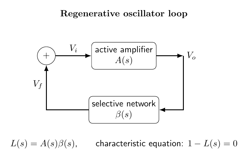
Throughout this discussion sinusoidal phasors use the convention $e^{j\omega t}$. Let $A(s)$ be the forward voltage gain and $\beta(s)$ the transfer function from output to the summing input. The sign at the summing junction is included in $\beta$, so the loop gain is
\[L(s)=A(s)\beta(s).\]Feedback equation and the characteristic equation
For an externally applied signal $V_s$ and regenerative feedback,
\[V_i=V_s+\beta V_o,\qquad V_o=A V_i.\]Eliminating $V_i$ gives
\[\boxed{\frac{V_o}{V_s}=\frac{A(s)}{1-A(s)\beta(s)}}.\]Natural oscillations are possible with $V_s=0$ only when a nonzero $V_o$ satisfies
\[\boxed{1-L(s)=0}.\]This is the characteristic equation of the closed loop. A sustained sinusoid of angular frequency $\omega_0$ corresponds, in the ideal linear description, to roots at $s=\pm j\omega_0$. Hence
\[L(j\omega_0)=1,\]or equivalently
\[\boxed{\lvert A(j\omega_0)\beta(j\omega_0)\rvert=1,\qquad \arg A(j\omega_0)+\arg\beta(j\omega_0)=2\pi n.}\]These are the magnitude and phase forms of the Barkhausen condition. They are necessary conditions for a steady sinusoid in the linearized loop, but are not by themselves a stability theorem. The locations of all characteristic roots and the nonlinear amplitude-control mechanism determine whether startup occurs and whether the final motion is stable.
Startup from noise and amplitude stabilization
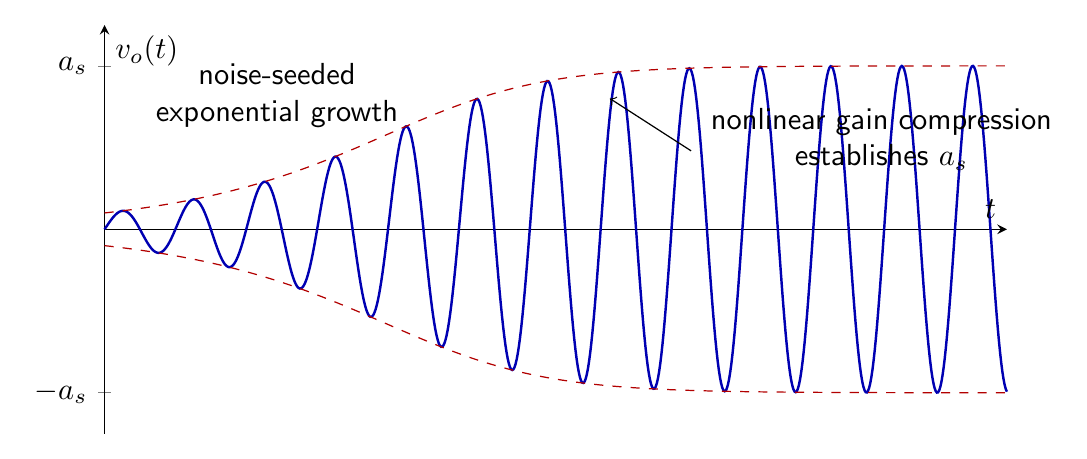
On switching on, thermal noise, switching transients and device noise contain small components over a broad frequency range. If the small-signal loop gain near one frequency obeys $\lvert L\rvert>1$ and has nearly zero loop phase, that component grows. For a narrow-band resonator the slowly varying envelope $a(t)$ may be written in the normal form
\[\frac{da}{dt}=\big[\mu-\nu a^2\big]a, \qquad \mu,\nu>0.\]When $a$ is small, $a\simeq a_0e^{\mu t}$; the origin is unstable. Growth stops at
\[\boxed{a_s=\sqrt{\frac{\mu}{\nu}}},\]where the effective large-signal loop gain has fallen to unity. Device saturation can provide this reduction but produces severe harmonics. Cleaner oscillators use automatic gain control, lamp or diode stabilization, field-effect resistance, or resonator nonlinearity so that the gain decreases smoothly with amplitude.
If $\lvert L\rvert<1$ at the selected frequency, disturbances decay. If $\lvert L\rvert=1$ only in an exactly linear, noiseless model, the final amplitude is undetermined by that model and depends on the initial condition. A realizable self-starting design therefore uses a small-signal gain slightly above the steady-state requirement and a controlled nonlinearity to restore unity loop gain.
Frequency selection and types of oscillators
Oscillators may be classified by waveform or by the frequency-selective element.
- RC sinusoidal oscillators use resistor-capacitor networks and are convenient from sub-hertz frequencies through the audio range. Phase-shift and Wien-bridge oscillators are principal examples.
- LC oscillators use an inductor-capacitor resonator, with $\omega_0\simeq1/\sqrt{LC}$, and are common at radio frequencies. Hartley and Colpitts circuits differ in how the reactive divider supplies feedback.
- Crystal oscillators exploit a piezoelectric mechanical resonance having very high quality factor $Q$, and therefore provide substantially better frequency stability.
- Relaxation oscillators repeatedly charge and discharge a capacitor between thresholds. They generate nonsinusoidal waveforms and are described by switching times rather than by a single linear resonance.
In a sinusoidal feedback oscillator, the phase condition ordinarily selects $\omega_0$. Write the loop phase as $\Phi(\omega,p)$, where $p$ is a component or environmental parameter. The equation $\Phi(\omega_0,p)=2\pi n$ gives, by implicit differentiation,
\[\boxed{\frac{d\omega_0}{dp}=- \frac{\partial\Phi/\partial p}{\partial\Phi/\partial\omega}\bigg\rvert_{\omega_0}}.\]A large loop phase slope $\lvert d\Phi/d\omega\rvert$ makes the selected frequency less sensitive to a given phase perturbation. This is why a high-$Q$ resonator improves short-term frequency discrimination.
Frequency and amplitude stability
Frequency stability is often specified by the fractional deviation
\[\boxed{S_f=\frac{\Delta f}{f_0}},\]over a stated time, temperature interval, supply range and load. The principal mechanisms are component tolerances and temperature coefficients, active-device phase shift, supply variation, resonator aging, mechanical vibration and load pulling. If $f=f(x_1,x_2,\ldots)$, small independent changes give
\[\frac{\Delta f}{f}\simeq \sum_i \frac{\partial\ln f}{\partial\ln x_i}\frac{\Delta x_i}{x_i}.\]For $f_0=(2\pi\sqrt{LC})^{-1}$,
\[\boxed{\frac{\Delta f_0}{f_0}\simeq-\frac12 \left(\frac{\Delta L}{L}+\frac{\Delta C}{C}\right)}.\]For an equal-component RC oscillator with $f_0=k/(RC)$,
\[\boxed{\frac{\Delta f_0}{f_0}\simeq-\frac{\Delta R}{R}-\frac{\Delta C}{C}}.\]Amplitude stability means that the limit-cycle amplitude changes little with supply, temperature, active-device parameters and load. Let the amplitude-dependent loop magnitude be $M(a)=\lvert A(a)\beta\rvert$. A steady amplitude $a_s$ satisfies $M(a_s)=1$. It is locally stable when an increase in amplitude makes the loop gain smaller:
\[\boxed{\left.\frac{dM}{da}\right\rvert_{a_s}<0.}\]If the derivative is positive, an amplitude perturbation grows. Very abrupt limiting provides stable amplitude but increases harmonic distortion; very weak limiting gives low distortion but slow recovery after disturbances. Practical design balances these effects.
Loop-gain response and phase margin interpretation
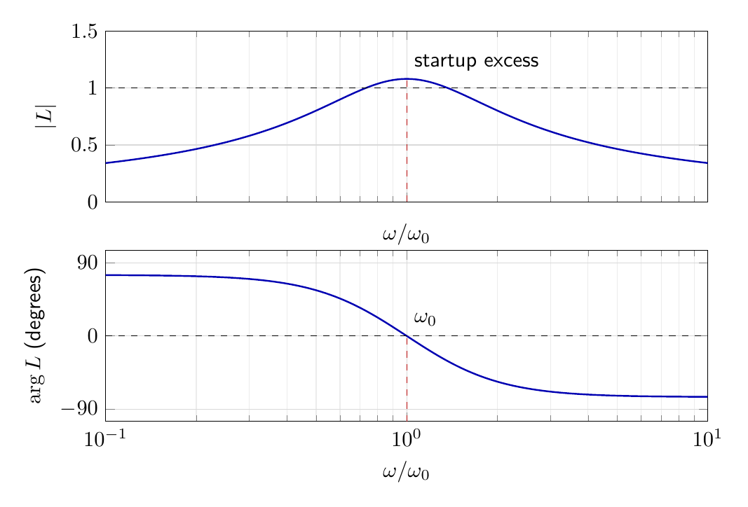
At the oscillation frequency, the Nyquist locus of $L(j\omega)$ passes through the point $+1$ for the positive-feedback convention used here. In the more usual negative-feedback convention the equivalent critical point is $-1$. Confusing these sign conventions is a common source of an erroneous extra $180^\circ$.
Near $\omega_0$, write
\[L(j\omega)\simeq[1+m(\omega)]e^{j\Phi(\omega)}.\]The gain excess $m(\omega_0)>0$ controls startup rate, while the phase slope controls frequency discrimination. In the plotted example, $\lvert L(\omega_0)\rvert=1.08$ at the zero-phase frequency: this is the small-signal startup value, not the final large-signal loop gain. As the oscillation grows, nonlinear gain compression reduces the effective fundamental loop magnitude from $1.08$ to unity. Unwanted frequencies must fail at least one Barkhausen condition. A loop response with multiple unity-gain, zero-phase crossings can support mode competition or mode hopping.
Pole motion and the onset of oscillation
The characteristic equation gives a more precise startup criterion than the isolated statement $\lvert L\rvert=1$. Let a design parameter $g$ represent amplifier gain. Below its critical value, the dominant conjugate poles may be written
\[s_{1,2}=-\sigma\pm j\omega_d,\qquad \sigma>0,\]so a disturbance contains the decaying factor $e^{-\sigma t}$. At critical gain the poles reach $s=\pm j\omega_0$. Increasing gain further moves them into the right half-plane in the linearized model and the corresponding component grows as $e^{\sigma_g t}$. A physical circuit cannot grow without limit; nonlinear gain reduction bends this linear instability into a stable finite-amplitude orbit. Thus gain above unity refers to the small-signal loop, whereas unity loop gain refers to the final fundamental component.
For a resonant mode with slowly varying complex amplitude $z$, an illustrative normal form is
\[\dot z=(\mu+j\Delta\omega)z-(\nu+j\kappa)\lvert z\rvert^2z.\]Writing $z=ae^{j\theta}$ gives
\[\dot a=(\mu-\nu a^2)a, \qquad \dot\theta=\Delta\omega-\kappa a^2.\]The real nonlinear coefficient $\nu$ stabilizes amplitude, whereas $\kappa$ describes amplitude-to-frequency conversion. Consequently an amplitude-control element may shift frequency if it also changes phase.
Linearizing the envelope about $a_s=\sqrt{\mu/\nu}$ gives
\[\frac{d(\delta a)}{dt}=-2\mu\,\delta a.\]Amplitude perturbations return with time constant $\tau_a=(2\mu)^{-1}$. Very small startup excess gives slow buildup and slow recovery; large excess gain shortens startup but drives the circuit more strongly into nonlinear operation.
Loaded resonator and energy balance
For a resonator storing average energy $W$ and losing energy $P_\ell$, its loaded quality factor is
\[Q_L=\omega_0\frac{W}{P_\ell}.\]The active circuit must deliver $P_\ell$ per unit time at steady state. Loading the output increases loss, lowers $Q_L$, changes the feedback fraction and can shift the phase condition. A buffer amplifier reduces load pulling by isolating the resonator from the external circuit. Noise perturbs both amplitude and phase; because phase has no restoring reference in a free-running oscillator, phase fluctuations accumulate and appear as spectral broadening or phase noise around the carrier.
The distinction between loaded and unloaded quality factor is essential. If a bare resonator loses power $P_i$ internally and coupling to the amplifier and load removes $P_e$, then
\[\frac1{Q_L}=\frac1{Q_i}+\frac1{Q_e}, \qquad Q_i=\omega_0\frac{W}{P_i},\quad Q_e=\omega_0\frac{W}{P_e}.\]Stronger coupling makes output extraction easier but lowers $Q_L$ and weakens frequency discrimination. The active circuit must replace both internal and externally extracted power.
Preparation questions
- Starting from the regenerative-feedback equation, derive the characteristic equation and state the Barkhausen conditions with an explicit sign convention.
- Explain why $\lvert A\beta\rvert=1$ does not by itself guarantee startup or a stable final amplitude.
- Derive the sensitivity of the oscillation frequency to a parameter through the loop-phase condition.
- Compare RC, LC, crystal and relaxation oscillators in terms of frequency selection and waveform.
- A resonator has $L=10\,\mathrm{mH}$ and $C=10\,\mathrm{nF}$. Estimate the fractional frequency shift when both components increase by $0.5\%$.
- Give the local condition on amplitude-dependent loop gain for a stable limit cycle and interpret it physically.


Discussion