

12 Jun 2026
Ferroelectricity: Dipole Theory, Classification, Properties and Applications
Mean-field and Landau theories of ferroelectric order, phase transitions, domains, hysteresis, crystal classes and applications.
A ferroelectric is a crystalline dielectric that possesses a spontaneous electric polarization $\mathbf P_s$ over a range of temperature and whose polarization direction can be reversed between symmetry-equivalent states by an applied electric field. The requirement of switchability distinguishes a ferroelectric from a material that is merely polar. The name reflects a thermodynamic and domain analogy with ferromagnetism; it does not imply the presence of iron.
At zero field, a macroscopic specimen may show little net polarization because it divides into domains with different directions of $\mathbf P_s$. Spontaneous polarization is a local equilibrium property of each domain. A sufficiently strong field changes the domain populations and can reverse the polar state.
Ferroelectricity occurs only in a polar crystallographic phase. Of the 32 crystallographic point groups, 21 are non-centrosymmetric, 20 of those are piezoelectric, and 10 are polar (pyroelectric). Ferroelectrics form the switchable subset of polar pyroelectric crystals:
\[\text{ferroelectric}\subset \text{pyroelectric}\subset \text{piezoelectric}\subset \text{non-centrosymmetric crystal}.\]Characteristic dielectric behaviour
The polarization and electric displacement in SI units are related by
\[\mathbf D=\varepsilon_0\mathbf E+\mathbf P.\]In the paraelectric phase and at a sufficiently weak field,
\[P_i=\varepsilon_0\chi_{ij}E_j.\]Near a ferroelectric transition, one or more components of the susceptibility become very large and strongly temperature dependent. Above the transition, many proper ferroelectrics approximately obey the Curie–Weiss law
\[\boxed{ \chi_e=\frac{C}{T-T_0}, \qquad \varepsilon_r\simeq\varepsilon_{\mathrm b}+\frac{C}{T-T_0}. }\]$C$ is the Curie constant, $T_0$ is the Curie–Weiss temperature, and $\varepsilon_{\mathrm b}$ is a comparatively slowly varying background permittivity. The observed transition temperature $T_c$ equals $T_0$ in an ideal continuous transition but generally exceeds it in a first-order transition.
Weiss dipole theory
The Weiss model describes a set of permanent or locally formed dipoles coupled through a mean internal field. Let each dipole have magnitude $\mu$, let $N$ be their number density, and take the effective field to be
\[\boxed{E_{\mathrm{eff}}=E+\lambda P.}\]The phenomenological constant $\lambda$ measures the cooperative interaction; in SI units it has units $\mathrm{m\,F^{-1}}$ so that $\lambda P$ has units $\mathrm{V\,m^{-1}}$. It is not generally equal to the Lorentz coefficient $1/(3\varepsilon_0)$ because short-range forces and lattice-mediated interactions are essential in real ferroelectrics.
For classical freely orientable dipoles, the self-consistency equation is
\[\boxed{ P=N\mu L\!\left[ \frac{\mu(E+\lambda P)}{k_{\mathrm B}T} \right], }\]where $L(x)=\coth x-1/x$ is the Langevin function. Even when $E=0$, this nonlinear equation can have solutions $P\ne0$ below a critical temperature.
Curie–Weiss law from the mean field
In the paraelectric weak-field region, $L(x)\simeq x/3$, and hence
\[P=\frac{N\mu^2}{3k_{\mathrm B}T}(E+\lambda P).\]Define the electric Curie constant
\[C=\frac{N\mu^2}{3\varepsilon_0k_{\mathrm B}}\]and the mean-field transition scale
\[T_0=\varepsilon_0\lambda C =\frac{N\mu^2\lambda}{3k_{\mathrm B}}.\]Solving for $P/E$ gives
\[P\left(1-\frac{T_0}{T}\right) =\frac{\varepsilon_0C}{T}E,\]and therefore
\[\boxed{ \chi_e=\frac{P}{\varepsilon_0E} =\frac{C}{T-T_0}. }\]The divergence is caused by positive feedback: a small polarization produces an internal field $\lambda P$, which aligns more dipoles. The independent-dipole Curie law $C/T$ is recovered when $\lambda=0$.
Spontaneous polarization in the Weiss approximation
For $E=0$, expand the Langevin function through cubic order:
\[P=N\mu\left[ \frac{\mu\lambda P}{3k_{\mathrm B}T} -\frac{1}{45} \left(\frac{\mu\lambda P}{k_{\mathrm B}T}\right)^3 +\cdots\right].\]For a non-zero solution, division by $P$ yields
\[1=\frac{T_0}{T} -\frac{N\mu^4\lambda^3}{45k_{\mathrm B}^3T^3}P_s^2+\cdots.\]Near $T_0$ from below,
\[P_s^2 =\frac{45k_{\mathrm B}^3T^2(T_0-T)} {N\mu^4\lambda^3},\]so $P_s\propto(T_0-T)^{1/2}$. The exponent $1/2$ is the mean-field critical exponent. The continuous-orientation Weiss model is useful for showing cooperative order, but real order–disorder ferroelectrics often have a discrete set of allowed dipole orientations, and displacive ferroelectrics require a lattice-mode description.
Landau theory of a proper ferroelectric
Landau theory uses symmetry and thermodynamics rather than a particular microscopic dipole model. Consider a uniaxial proper ferroelectric with scalar polarization $P$ along its polar axis. At prescribed electric field, write the appropriate Landau thermodynamic potential (electric enthalpy density) as
\[\boxed{ f(P,T,E)=f_0(T) +\frac{\alpha}{2}P^2 +\frac{b}{4}P^4 +\frac{c}{6}P^6-EP, }\]where
\[\alpha=a(T-T_0),\qquad a>0,\qquad c>0.\]Only even powers occur at $E=0$ when the paraelectric phase has inversion symmetry, because $P$ and $-P$ must have the same energy. The term $-EP$ is the work of the external field. Since $f$ is measured in $\mathrm{J\,m^{-3}}$ and $P$ in $\mathrm{C\,m^{-2}}$, the SI units are
\[[\alpha]=\mathrm{V\,m\,C^{-1}},\quad [b]=\mathrm{V\,m^5\,C^{-3}},\quad [c]=\mathrm{V\,m^9\,C^{-5}}.\]Equilibrium requires
\[\frac{\partial f}{\partial P}=0,\]which gives the constitutive equation
\[\boxed{E=\alpha P+bP^3+cP^5.}\]Stability further requires $\partial^2f/\partial P^2>0$:
\[\alpha+3bP^2+5cP^4>0.\]Continuous transition: $b>0$
For a continuous transition, the sixth-order term is not needed for stability close to $T_0$, and one may set $c=0$. At $E=0$,
\[P(\alpha+bP^2)=0.\]For $T>T_0$, $\alpha>0$ and the stable solution is $P=0$. For $T<T_0$, $\alpha<0$ and the two symmetry-related stable states are
\[\boxed{ P_s=\pm\sqrt{-\frac{\alpha}{b}} =\pm\sqrt{\frac{a(T_0-T)}{b}}. }\]Above $T_0$, differentiate $E=\alpha P+bP^3$ at $P=0$:
\[\chi_+ =\frac{1}{\varepsilon_0} \left(\frac{\partial P}{\partial E}\right)_{E=0} =\frac{1}{\varepsilon_0a(T-T_0)}.\]Thus $C_+=1/(\varepsilon_0a)$. Below the transition, evaluate the curvature at $P=P_s$:
\[\left.\frac{\partial E}{\partial P}\right|_{P_s} =\alpha+3bP_s^2=-2\alpha=2a(T_0-T).\]Therefore the intrinsic single-domain susceptibility is
\[\boxed{ \chi_-= \frac{1}{2\varepsilon_0a(T_0-T)}. }\]Mean-field Landau theory predicts a factor-of-two ratio between the Curie constants extrapolated from the paraelectric and ferroelectric sides. Domain-wall motion can make the measured low-frequency response much larger than this intrinsic value.
The entropy density difference between the polar and nonpolar solutions is
\[\Delta s=-\frac{\partial(f_s-f_0)}{\partial T} =-\frac{a}{2}P_s^2,\]which approaches zero continuously at $T_0$. There is no latent heat in this ideal second-order transition.
First-order transition: $b<0$, $c>0$
When $b<0$, the sixth-order term is required to bound the free energy. A non-zero minimum can become globally stable while $\alpha$ is still positive. At zero field, a polar stationary state satisfies
\[\alpha+bP^2+cP^4=0.\]At the transition, the polar and nonpolar phases have equal free energy:
\[\frac{\alpha}{2}P^2 +\frac{b}{4}P^4 +\frac{c}{6}P^6=0.\]Solving these two conditions gives
\[\boxed{ P_{\mathrm{jump}}^2=-\frac{3b}{4c}, \qquad \alpha_c=\frac{3b^2}{16c}. }\]Hence
\[\boxed{ T_c=T_0+\frac{3b^2}{16ac}>T_0. }\]The polarization changes discontinuously, metastable minima occur over a finite temperature interval, and the transition has latent heat. The distinction $T_c>T_0$ explains why the Curie–Weiss extrapolation can vanish below the measured transition temperature.
Hysteresis and coercive field
Below the transition, $f(P)$ has symmetry-related minima. Sweeping the electric field tilts the free energy through $-EP$. If a state remains in a metastable local minimum until that minimum loses stability, the calculated $P(E)$ curve is hysteretic.
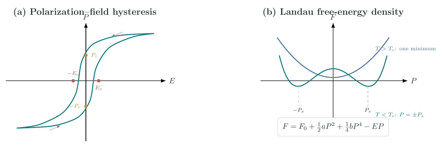
For the quartic model below $T_0$,
\[E(P)=\alpha P+bP^3, \qquad \alpha<0,\quad b>0.\]The metastability limit occurs where
\[\frac{dE}{dP}=\alpha+3bP^2=0.\]Thus
\[P_{\mathrm{sp}}^2=\frac{|\alpha|}{3b}\]and the magnitude of the ideal homogeneous, or intrinsic, coercive field is
\[\boxed{ |E_c^{\mathrm{int}}| =\frac{2|\alpha|^{3/2}}{3\sqrt{3b}}. }\]An experimental hysteresis loop is characterized by the remanent polarization $P_r$ at $E=0$, the coercive fields at which the macroscopic polarization reverses, and the saturation polarization at high field. Real coercive fields are usually far below the homogeneous Landau value because switching begins by nucleation and motion of domain walls at defects, surfaces and electrodes. A measured loop can also contain leakage-current and dielectric-loss contributions; a loop-like trace alone is not sufficient proof of ferroelectric switching.
Ferroelectric domains
A uniformly polarized finite specimen produces bound surface charge
\[\sigma_b=\mathbf P_s\cdot\hat{\mathbf n},\]and an associated depolarizing field. The electrostatic energy can be reduced by forming domains whose polarizations point in different allowed directions. Domain formation costs domain-wall energy, so equilibrium domain size results from competition between wall and electrostatic or elastic energies.
- A $180^\circ$ domain wall separates antiparallel polarization states. It changes the bound charge pattern without changing the spontaneous strain orientation.
- A non-$180^\circ$ wall, such as a $90^\circ$ wall in a tetragonal perovskite, separates states with different polarization and strain directions. Elastic compatibility is therefore important.
To describe a spatially varying polarization, Landau–Ginzburg theory adds a gradient term,
\[f_{\mathrm G}=f(P)+\frac{g}{2}(\nabla P)^2, \qquad g>0.\]For a one-dimensional $180^\circ$ wall in the quartic theory at zero field,
\[g\frac{d^2P}{dx^2}=\alpha P+bP^3.\]With $\alpha<0$ and $P_s=\sqrt{\lvert\alpha\rvert/b}$, the wall connecting $-P_s$ and $+P_s$ is
\[\boxed{ P(x)=P_s\tanh\left(\frac{x}{\delta}\right), \qquad \delta=\sqrt{\frac{2g}{|\alpha|}}. }\]Its ideal wall energy per unit area is
\[\boxed{ \sigma_w=\frac{2\sqrt2}{3} \frac{|\alpha|^{3/2}\sqrt g}{b}. }\]Free charge supplied by electrodes, mobile carriers or adsorbates can screen the bound charge. In ultrathin films, incomplete screening produces a strong depolarizing field and may suppress the single-domain state or favour closure domains.
Coupling to strain
Ferroelectric polarization couples to mechanical deformation. In a centrosymmetric paraelectric reference phase, the lowest electrostrictive coupling is even in $P$. For one strain component $u$,
\[f_{\mathrm{el}}=\frac{K}{2}u^2-q\,uP^2-\sigma u,\]where $K$ is an elastic modulus, $q$ an electrostrictive coefficient and $\sigma$ applied stress. At zero stress, minimization gives
\[u=\frac{q}{K}P^2.\]In the polar phase, expand $P=P_s+\delta P$. Then $P^2$ contains the term $2P_s\delta P$, producing a response linear in the small electric field. This is the symmetry-based phenomenological origin of piezoelectricity in the ferroelectric phase. Eliminating strain also renormalizes the quartic coefficient,
\[b_{\mathrm{eff}}=b-\frac{2q^2}{K}\]for the normalization used above; sufficiently strong coupling can drive an otherwise continuous transition first order.
Displacive and order–disorder mechanisms
The labels displacive and order–disorder refer to microscopic mechanisms, not to whether the transition is first or second order.
Displacive ferroelectrics
In a displacive transition, the high-symmetry phase has ions centred near symmetric positions. A zone-centre transverse optical lattice mode softens as the transition is approached, and its static displacement creates the polar structure. On the paraelectric side of an ideal continuous soft-mode transition, schematically,
\[\omega_{\mathrm{TO}}^2(T)\simeq A(T-T_0).\]For a first-order displacive transition, the soft-mode frequency generally remains finite at the observed $T_c>T_0$ and extrapolates towards zero at the lower Curie–Weiss temperature $T_0$. The mode effective charge makes the soft coordinate couple to the electric field. The Lyddane–Sachs–Teller relation for a single dominant polar branch,
\[\frac{\varepsilon(0)}{\varepsilon_\infty} =\frac{\omega_{\mathrm{LO}}^2}{\omega_{\mathrm{TO}}^2},\]connects softening of $\omega_{\mathrm{TO}}$ with the large static permittivity. BaTiO$_3$, PbTiO$_3$ and KNbO$_3$ are standard predominantly displacive proper ferroelectrics, although local off-centring can make the microscopic behaviour more mixed than an ideal soft-mode picture.
Order–disorder ferroelectrics
In an order–disorder transition, local dipoles or polar structural units already exist above $T_c$ but occupy symmetry-equivalent orientations randomly. Below $T_c$, cooperative interactions select an ordered population. Their dynamics is commonly relaxational rather than a purely harmonic soft phonon. KH$_2$PO$_4$ (KDP), triglycine sulfate (TGS) and NaNO$_2$ are representative order–disorder ferroelectrics. The Weiss dipole equation captures the central self-consistency idea, although microscopic models use discrete orientations and material-specific interactions.
Displacive and order–disorder behaviour are limiting descriptions. A real crystal may show both a soft phonon and persistent local distortions.
Proper, improper and hybrid-improper ferroelectrics
This classification concerns the role of polarization in the phase transition and is independent of the displacive/order–disorder distinction.
Proper ferroelectrics
In a proper ferroelectric, polarization is the primary order parameter. Its quadratic stiffness tends towards zero at the transition, which usually produces a strong dielectric anomaly. BaTiO$_3$, PbTiO$_3$, KDP and TGS are proper ferroelectrics even though the first two are mainly displacive and the latter examples are mainly order–disorder.
Improper ferroelectrics
In an improper ferroelectric, the primary order parameter $Q$ is a nonpolar structural distortion, magnetic order, charge order, or another collective variable. Polarization is secondary and is induced by a symmetry-allowed coupling. A schematic free energy is
\[f(Q,P)=f_Q(Q)+\frac{P^2}{2\varepsilon_0\chi_0} +\gamma P Q^n+\cdots.\]Minimizing over $P$ gives
\[P=-\varepsilon_0\chi_0\gamma Q^n.\]The polarization therefore appears because $Q$ condenses; its own polar stiffness need not soften. Hexagonal YMnO$_3$ is a widely studied geometric improper ferroelectric, where a nonpolar structural trimerization is primary.
Hybrid-improper ferroelectrics
In a hybrid-improper ferroelectric, two distinct nonpolar distortions $Q_1$ and $Q_2$ combine through a trilinear invariant,
\[f_{\mathrm{tri}}=\gamma P Q_1Q_2.\]Then $P\propto Q_1Q_2$. Layered perovskites such as Ca$_3$Ti$_2$O$_7$ provide representative examples, with two octahedral rotation patterns combining to induce polarization.
Other useful ferroelectric classifications
Classification axes should not be confused with one another:
| Classification | Meaning | Representative examples |
|---|---|---|
| Uniaxial | $\mathbf P_s$ is restricted to one crystallographic axis, with two opposite states | TGS, KDP, LiNbO$_3$ |
| Multiaxial | Several symmetry-related polar axes are possible | BaTiO$_3$, KNbO$_3$, Pb(Zr,Ti)O$_3$ |
| Proper | $P$ is the primary order parameter | BaTiO$_3$, PbTiO$_3$, KDP |
| Improper | A nonpolar primary order induces $P$ | hexagonal YMnO$_3$ |
| Hybrid improper | Two nonpolar modes induce $P$ through $PQ_1Q_2$ | Ca$_3$Ti$_2$O$_7$ |
| Displacive | A polar lattice displacement or soft mode develops | PbTiO$_3$, BaTiO$_3$ |
| Order–disorder | Pre-existing local dipoles become orientationally ordered | KDP, TGS, NaNO$_2$ |
An antiferroelectric has oppositely polarized sublattices with zero net polarization in its ground state and can undergo a field-induced transition to a polar state, often giving a double hysteresis loop. A ferrielectric has antiparallel unequal sublattice polarizations and therefore a non-zero resultant. These are ordered polar-sublattice states, but they are not synonyms for an ordinary ferroelectric domain arrangement.
Properties and applications
The coupled electrical, mechanical, thermal and optical responses of ferroelectrics support several device classes.
High-permittivity capacitors
Large susceptibility near a polar instability makes BaTiO$_3$-based ceramics useful in multilayer ceramic capacitors. Compositional control, grain size and dopants broaden and stabilize the useful temperature range. Ferroelectric capacitors are nonlinear, so capacitance depends on field amplitude, bias and frequency.
Non-volatile polarization memory
Two remanent polarization states can encode binary information. Ferroelectric random-access memory uses switching charge for readout, while ferroelectric field-effect devices use polarization charge to modulate a semiconductor channel. Retention, fatigue, imprint, leakage and scaling of the depolarizing field are central materials issues.
Piezoelectric transducers and actuators
A poled ferroelectric ceramic has a net piezoelectric response. Lead zirconate titanate, Pb(Zr,Ti)O$_3$ (PZT), is used in ultrasound transducers, sonar, precision positioning, accelerometers and vibration control. Domain-wall motion enhances the response but introduces nonlinearity and hysteresis. Lead-free alternatives are pursued because of environmental restrictions on lead.
Pyroelectric and electrocaloric devices
The pyroelectric coefficient
\[p=\left(\frac{\partial P_s}{\partial T}\right)_{E,\sigma}\]relates a temperature change to surface charge and is used in infrared detectors and thermal sensors. Under suitable conditions, an applied-field change produces an adiabatic temperature change, the electrocaloric effect.
Electro-optic and nonlinear-optical devices
Polarization and strain alter the optical indicatrix. LiNbO$_3$ is widely used for electro-optic modulators, frequency conversion and waveguides. The lack of inversion symmetry also permits second-order nonlinear-optical processes.
Tunable dielectric and microwave components
The field dependence of permittivity enables tunable capacitors, phase shifters and filters. Low dielectric loss is essential at microwave frequencies, so the composition and defect chemistry must be optimized separately from maximizing the static permittivity.
Worked Landau examples
Continuous transition
Consider the illustrative SI coefficients
\[a=3.00\times10^5\ \mathrm{V\,m\,C^{-1}\,K^{-1}}, \qquad b=2.00\times10^9\ \mathrm{V\,m^5\,C^{-3}},\]with $T_0=400\ \mathrm K$. At $T=380\ \mathrm K$,
\[\alpha=a(T-T_0)=-6.00\times10^6\ \mathrm{V\,m\,C^{-1}}.\]The spontaneous polarization is
\[P_s=\sqrt{\frac{|\alpha|}{b}} =5.48\times10^{-2}\ \mathrm{C\,m^{-2}}.\]The intrinsic small-signal susceptibility in one domain is
\[\chi_-=\frac{1}{2\varepsilon_0|\alpha|} =9.41\times10^3.\]The homogeneous Landau coercive field is
\[|E_c^{\mathrm{int}}| =\frac{2|\alpha|^{3/2}}{3\sqrt{3b}} =1.26\times10^5\ \mathrm{V\,m^{-1}}.\]This is a thermodynamic spinodal field for a spatially uniform model, not a prediction of the much smaller defect-controlled coercive field of a macroscopic specimen.
First-order transition
Take
\[a=3.00\times10^5\ \mathrm{V\,m\,C^{-1}\,K^{-1}},\] \[b=-4.00\times10^8\ \mathrm{V\,m^5\,C^{-3}}, \qquad c=6.00\times10^9\ \mathrm{V\,m^9\,C^{-5}}.\]The shift of the transition above the Curie–Weiss temperature is
\[T_c-T_0=\frac{3b^2}{16ac}=16.7\ \mathrm K,\]and the discontinuous polarization at coexistence is
\[P_{\mathrm{jump}} =\sqrt{-\frac{3b}{4c}} =2.24\times10^{-1}\ \mathrm{C\,m^{-2}}.\]Both phases are equilibrium stationary states at $T_c$, but the finite $P_{\mathrm{jump}}$ identifies the transition as first order.
Preparation questions
- State the defining conditions for ferroelectricity and distinguish ferroelectric, pyroelectric and piezoelectric crystals.
- Starting from the Weiss effective field $E+\lambda P$, derive the Curie–Weiss law and identify the Curie constant and Curie–Weiss temperature.
- Use the cubic expansion of the Langevin function to obtain the temperature dependence of the spontaneous polarization near the mean-field transition.
- Develop Landau theory for a continuous ferroelectric transition and derive $P_s(T)$ and the susceptibilities above and below $T_c$.
- For $b<0$ and $c>0$, derive $P_{\mathrm{jump}}^2=-3b/(4c)$ and $T_c-T_0=3b^2/(16ac)$.
- Derive the intrinsic coercive field of the quartic Landau model and explain why measured coercive fields are generally smaller.
- Obtain the profile, width and energy of a one-dimensional $180^\circ$ domain wall in Landau–Ginzburg theory.
- Distinguish displacive and order–disorder ferroelectrics, giving representative crystals of each type.
- Distinguish proper, improper and hybrid-improper ferroelectricity by writing appropriate free-energy couplings.
- Explain the origin of depolarizing fields and the formation of ferroelectric domains.
- Discuss the dielectric, piezoelectric, pyroelectric and electro-optic properties that underlie major ferroelectric applications.
- A proper ferroelectric has $a=2.5\times10^5\ \mathrm{V\,m\,C^{-1}\,K^{-1}}$, $b=1.2\times10^9\ \mathrm{V\,m^5\,C^{-3}}$ and $T_0=350\ \mathrm K$. Calculate $P_s$ and the intrinsic susceptibility at $T=330\ \mathrm K$.


Discussion