

05 Jun 2026
Lorentz Local Field and the Clausius–Mossotti Equation
Lorentz-cavity construction, molecular field, Clausius–Mossotti and Lorentz–Lorenz relations, stability, and the polarization catastrophe.
The macroscopic electric field is an average over a region containing many microscopic charges. An atom or molecule does not respond directly to this spatial average: it responds to the local field at its own site. The Lorentz construction relates these two fields for an isotropic or cubic dielectric and leads to the Clausius–Mossotti equation.
All formulas use SI units. The derivation is electrostatic, assumes linear polarizability, and treats the dielectric as homogeneous on the scale of a fictitious cavity. The field $\mathbf E$ denotes the macroscopic internal field, not the externally imposed field before depolarization corrections.
Macroscopic field and local field
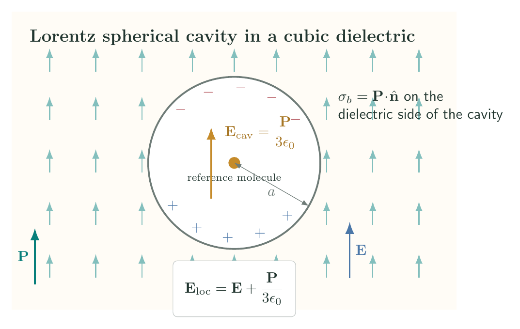
Let the dielectric be uniformly polarized, and remove a small spherical region centred on the microscopic unit whose response is being calculated. The radius of this Lorentz cavity is chosen to be large compared with an interatomic spacing but small compared with the scale on which $\mathbf P$ changes.
The local field can be separated conceptually as
\[\mathbf E_{\mathrm{loc}} =\mathbf E+\mathbf E_{\mathrm{cav}}+\mathbf E_{\mathrm{near}}.\]Here $\mathbf E$ is the field produced by all free and bound charges when polarization is treated as a smooth continuum. The term $\mathbf E_{\mathrm{cav}}$ corrects for removing the continuum polarization from the spherical cavity. The term $\mathbf E_{\mathrm{near}}$ is the discrete field of the actual dipoles inside the region that was excluded from the continuum calculation.
For an atom at a site of cubic symmetry, the vector sum $\mathbf E_{\mathrm{near}}$ vanishes. Dipoles related by the cubic point group make cancelling contributions. This cancellation is not generally valid at a surface, at a defect, or in a noncubic lattice.
Field of the Lorentz cavity
Take $\mathbf P=P\hat{\mathbf z}$. The unit normal directed outward from the dielectric at the inner wall of the spherical cavity is $-\hat{\mathbf r}$. The bound surface-charge density on the wall is therefore
\[\sigma_b=\mathbf P\boldsymbol\cdot(-\hat{\mathbf r})=-P\cos\theta.\]For an area element $da=R^2\sin\theta\,d\theta\,d\phi$, the field at the centre points from the element toward the centre. Its $z$ component is
\[dE_z =\frac{1}{4\pi\epsilon_0} \frac{\sigma_b\,da}{R^2}(-\cos\theta) =\frac{P}{4\pi\epsilon_0}\cos^2\theta\sin\theta\,d\theta\,d\phi.\]Integration over the spherical wall gives
\[\begin{aligned} E_{\mathrm{cav},z} &=\frac{P}{4\pi\epsilon_0} \int_0^{2\pi}d\phi \int_0^\pi\cos^2\theta\sin\theta\,d\theta\\ &=\frac{P}{4\pi\epsilon_0}(2\pi)\left(\frac23\right) =\frac{P}{3\epsilon_0}. \end{aligned}\]Thus, for a cubic dielectric,
\[\boxed{\mathbf E_{\mathrm{loc}} =\mathbf E+\frac{\mathbf P}{3\epsilon_0}}.\]The sign is positive: the cavity-wall field is parallel to the polarization. This Lorentz field $\mathbf P/(3\epsilon_0)$ should not be confused with the depolarization field of the outer specimen, which opposes $\mathbf P$ and is already included in the macroscopic internal field $\mathbf E$.
Clausius–Mossotti equation
Suppose there are $N$ identical microscopic units per unit volume and each has isotropic polarizability $\alpha$. The induced dipole and polarization are
\[\mathbf p=\alpha\mathbf E_{\mathrm{loc}}, \qquad \mathbf P=N\mathbf p.\]Using the Lorentz field,
\[\mathbf P=N\alpha\left(\mathbf E+\frac{\mathbf P}{3\epsilon_0}\right).\]Collecting the terms proportional to $\mathbf P$,
\[\left(1-\frac{N\alpha}{3\epsilon_0}\right)\mathbf P =N\alpha\mathbf E.\]Since $\mathbf P=\epsilon_0\chi_e\mathbf E$,
\[\boxed{\chi_e= \frac{N\alpha/\epsilon_0}{1-N\alpha/(3\epsilon_0)}}.\]With $\epsilon_r=1+\chi_e$, define
\[x=\frac{N\alpha}{3\epsilon_0}.\]Then
\[\epsilon_r=1+\frac{3x}{1-x} =\frac{1+2x}{1-x}.\]Solving this relation for $x$ yields the Clausius–Mossotti equation,
\[\boxed{ \frac{\epsilon_r-1}{\epsilon_r+2} =\frac{N\alpha}{3\epsilon_0} }.\]The result contains the local-field correction to the dilute relation $\chi_e=N\alpha/\epsilon_0$. Expanding for $x\ll1$,
\[\chi_e=3x(1+x+x^2+\cdots) =\frac{N\alpha}{\epsilon_0} +\frac{N^2\alpha^2}{3\epsilon_0^2}+\cdots.\]The first term is the dilute result and the remaining terms are the Lorentz mean-field feedback.
Mixtures and molar polarization
If species $s$ have number densities $N_s$ and scalar polarizabilities $\alpha_s$, all species experience the same Lorentz field under the assumptions of the model. Hence
\[\mathbf P=\sum_sN_s\alpha_s \left(\mathbf E+\frac{\mathbf P}{3\epsilon_0}\right),\]and
\[\boxed{ \frac{\epsilon_r-1}{\epsilon_r+2} =\frac{1}{3\epsilon_0}\sum_sN_s\alpha_s }.\]For a pure substance of mass density $\rho_m$ and molar mass $M$, the number density is
\[N=\frac{N_A\rho_m}{M}.\]The molar polarization is therefore
\[\boxed{ P_m\equiv\frac{M}{\rho_m} \frac{\epsilon_r-1}{\epsilon_r+2} =\frac{N_A\alpha}{3\epsilon_0} }.\]For a transparent nonmagnetic material at frequencies where only electronic polarization follows the field and absorption is negligible, $n^2\simeq\epsilon_r$. The corresponding optical form is the Lorentz–Lorenz relation,
\[\boxed{ \frac{n^2-1}{n^2+2} =\frac{N\alpha_{\mathrm{el}}}{3\epsilon_0} }.\]It must not be used inside an absorption band, where $n$ and $\epsilon_r$ are complex and strongly frequency dependent.
Stability formulation of the molecular field
The Clausius–Mossotti denominator can be understood from a mean-field free-energy density. If $P=Np$, the reversible energy needed to induce a dipole $p$ in each of $N$ independent units is
\[f_{\mathrm{self}}=N\frac{p^2}{2\alpha} =\frac{P^2}{2N\alpha}.\]The Lorentz molecular-field interaction has the mean-field energy density
\[f_{\mathrm{L}}=-\frac{P^2}{6\epsilon_0}.\]The factor $1/2$ avoids double counting the mutual dipole interaction: differentiating $f_{\mathrm L}$ with respect to $P$ produces the local feedback field $P/(3\epsilon_0)$. At prescribed macroscopic field $E$ along the polarization, the electric enthalpy density of the linear model is
\[f(P;E)=\frac{P^2}{2N\alpha} -\frac{P^2}{6\epsilon_0}-EP.\]Stationarity gives
\[\frac{\partial f}{\partial P} =\left(\frac{1}{N\alpha}-\frac{1}{3\epsilon_0}\right)P-E=0,\]or
\[P=N\alpha\left(E+\frac{P}{3\epsilon_0}\right),\]which is precisely the Lorentz self-consistency equation.
The curvature at $P=0$ is
\[\frac{\partial^2f}{\partial P^2} =\frac{1}{N\alpha}-\frac{1}{3\epsilon_0} =\frac{1-x}{N\alpha}.\]The unpolarized state is stable only when
\[\boxed{x=\frac{N\alpha}{3\epsilon_0}<1}.\]Clausius–Mossotti catastrophe
As $x\to1^-$,
\[\chi_e=\frac{3x}{1-x}\longrightarrow+\infty, \qquad \epsilon_r=\frac{1+2x}{1-x}\longrightarrow+\infty.\]At $x=1$, the restoring curvature of the quadratic free energy vanishes. An infinitesimal macroscopic field then produces an unlimited polarization in the linear model. This singularity is called the Clausius–Mossotti catastrophe or polarization catastrophe.
For $x>1$, the quadratic coefficient is negative, so $P=0$ is unstable and the purely quadratic model is unbounded below. The formal negative value of $\epsilon_r=(1+2x)/(1-x)$ is not a valid equilibrium permittivity of the assumed insulating phase. It signals failure of the linear independent-dipole model.
A stable nonlinear theory must retain higher powers of $P$. For example,
\[f(P;0)=\frac12AP^2+\frac14bP^4, \qquad A=\frac{1}{N\alpha}-\frac{1}{3\epsilon_0}, \qquad b>0.\]When $A<0$, minimization gives
\[P\left(A+bP^2\right)=0,\]and the stable zero-field solutions are
\[P_s=\pm\sqrt{-\frac{A}{b}}.\]This mean-field regularization shows how the catastrophe can be associated with the onset of spontaneous polarization, but quantitative ferroelectric behaviour requires crystal-specific short-range forces, anharmonicity, domains, and tensor order parameters.
For permanent dipoles of magnitude $p_0$ in the weak-field, high-temperature limit, orientational averaging gives
\[\alpha_{\mathrm{or}}=\frac{p_0^2}{3k_BT}.\]If this is the only polarizability, the instability condition becomes
\[\frac{Np_0^2}{9\epsilon_0k_BT_C}=1,\]so the mean-field critical temperature is
\[T_C=\frac{Np_0^2}{9\epsilon_0k_B}.\]Above $T_C$,
\[\chi_e=\frac{3T_C}{T-T_C},\]which has Curie–Weiss form. The numerical coefficient is model dependent because the Lorentz field is not an exact treatment of the strongly correlated local environment in a real ferroelectric.
Range of validity
The Clausius–Mossotti relation assumes isotropic scalar polarizability, a spherical Lorentz cavity, cubic symmetry or an isotropic disordered medium, linear response, negligible spatial dispersion, and vanishing near-field lattice sum. It is most reliable for dilute gases and approximately isotropic nonpolar materials.
It can fail for strongly polar liquids, hydrogen-bonded systems, low-symmetry crystals, ionic crystals with collective optical modes, materials close to a ferroelectric transition, and heterogeneous samples dominated by interfaces. In such cases the microscopic response is correlated, and a scalar independent-unit polarizability is insufficient.
Numerical example and distance from instability
Let the polarizability volume be
\[a=\frac{\alpha}{4\pi\epsilon_0}=2.00\ \text{\AA}^3 =2.00\times10^{-30}\ \mathrm{m^3},\]and let $N=2.50\times10^{28}\ \mathrm{m^{-3}}$. Then
\[x=\frac{N\alpha}{3\epsilon_0} =\frac{4\pi Na}{3}=0.2094.\]The predicted relative permittivity is
\[\epsilon_r=\frac{1+2x}{1-x}=1.795.\]For the same microscopic polarizability, the formal critical density is
\[N_c=\frac{3\epsilon_0}{\alpha} =\frac{3}{4\pi a} =1.19\times10^{29}\ \mathrm{m^{-3}}.\]The stated density has $N/N_c=x=0.2094$, so it lies well inside the stable range of the mean-field model.
Preparation questions
- Distinguish the macroscopic internal field, Lorentz cavity field, near field, depolarization field, and local field.
- Calculate the electric field at the centre of a spherical cavity in a uniformly polarized dielectric and explain its sign.
- Derive the Clausius–Mossotti equation from $p=\alpha E_{\mathrm{loc}}$.
- Obtain the molar-polarization and Lorentz–Lorenz forms of the relation, stating their domains of validity.
- Derive the Clausius–Mossotti susceptibility as a geometric series and interpret the local-field feedback terms.
- Construct the quadratic mean-field free energy and prove that stability requires $N\alpha/(3\epsilon_0)<1$.
- Explain the Clausius–Mossotti catastrophe and show how a positive quartic term regularizes the instability.
- For permanent dipoles, derive the mean-field critical temperature and the Curie–Weiss susceptibility above it.


Discussion