

17 May 2026
Phonon Density of States and Van Hove Singularities
Mode counting, constant-frequency surfaces, Debye density of states, dimensional dependence, and Van Hove critical points.
A phonon dispersion relation assigns a frequency $\omega_{\mathbf q s}$ to every allowed wavevector $\mathbf q$ and branch $s$. The phonon density of states reorganizes this information according to frequency: it gives the number of normal modes in a specified frequency interval, irrespective of where those modes occur in the Brillouin zone.
Unless explicitly stated otherwise, the density of states below is defined per unit angular frequency. A density per hertz differs by a factor of $2\pi$.
Definition and normalization
For a crystal containing $N$ primitive cells and $r$ atoms per primitive cell, define
\[\boxed{ g(\omega)=\sum_{\mathbf q s} \delta(\omega-\omega_{\mathbf q s}). }\]The number of modes between $\omega$ and $\omega+d\omega$ is $g(\omega)d\omega$. The integrated density of states is
\[\mathcal N(\omega) =\int_0^\omega g(\omega')\,d\omega' =\sum_{\mathbf q s} \Theta(\omega-\omega_{\mathbf q s}).\]Because there are $N$ allowed wavevectors in each branch and $3r$ branches,
\[\boxed{ \int_0^\infty g(\omega)\,d\omega=3rN. }\]The three exact rigid-translation modes at $\mathbf q=0$ are included in this normalization. Their weight is $3/(3rN)=1/(rN)$, so only their fractional contribution vanishes in the thermodynamic limit. The density per unit volume is
\[\mathfrak g(\omega)=\frac{g(\omega)}{V}.\]For Born–von Karman boundary conditions,
\[\sum_{\mathbf q} \longrightarrow \frac{V}{(2\pi)^3} \int_{\mathrm{BZ}}d^3q,\]and hence
\[\boxed{ \mathfrak g(\omega) =\frac{1}{(2\pi)^3} \sum_s\int_{\mathrm{BZ}} d^3q\, \delta(\omega-\omega_{\mathbf q s}). }\]Every branch must be included separately, including degeneracies. Three-dimensional branch crossings do not double count states: each eigenvalue of the dynamical matrix contributes one branch at each $\mathbf q$.
Constant-frequency-surface formula
For a fixed branch, the equation
\[\omega_{\mathbf q s}=\omega\]defines one or more surfaces in reciprocal space. Introduce local coordinates with one coordinate normal to a constant-frequency surface. The volume element is
\[d^3q=dS\,dq_\perp,\]and, locally,
\[d\omega =\left\lvert\nabla_{\mathbf q}\omega_{\mathbf q s}\right\rvert dq_\perp.\]Using the delta-function transformation gives
\[\boxed{ \mathfrak g(\omega) =\frac{1}{(2\pi)^3} \sum_s \int_{S_s(\omega)} \frac{dS} {\left\lvert\nabla_{\mathbf q} \omega_{\mathbf q s}\right\rvert}. }\]Since
\[\mathbf v_g(\mathbf q,s) =\nabla_{\mathbf q}\omega_{\mathbf q s},\]regions of small group velocity contribute strongly to the density of states. A flat branch can therefore produce a large spectral peak even if it occupies a modest region of reciprocal space.
In $d$ spatial dimensions the corresponding result is
\[\frac{g_d(\omega)}{V_d} =\frac{1}{(2\pi)^d} \sum_s\int d^dq\, \delta(\omega-\omega_{\mathbf q s}).\]For an isotropic linear branch $\omega=vq$,
\[\frac{g_d(\omega)}{V_d} =\frac{S_{d-1}}{(2\pi)^d} \frac{\omega^{d-1}}{v^d},\]where
\[S_{d-1}=\frac{2\pi^{d/2}}{\Gamma(d/2)}\]is the area of a unit $(d-1)$-sphere. Thus a linear acoustic branch gives
\[g_1(\omega)\propto\omega^0,\qquad g_2(\omega)\propto\omega,\qquad g_3(\omega)\propto\omega^2.\]Debye density of states
At sufficiently small $\mathbf q$, a three-dimensional crystal has one longitudinal and two transverse acoustic branches. In an isotropic approximation,
\[\omega_L=v_Lq, \qquad \omega_{T1}=\omega_{T2}=v_Tq.\]The number of wavevectors in a spherical shell of radius $q$ and thickness $dq$ is
\[\frac{V}{(2\pi)^3}4\pi q^2dq.\]For one linear branch, $q=\omega/v_s$ and $dq=d\omega/v_s$, so
\[g_s(\omega) =\frac{V\omega^2}{2\pi^2v_s^3}.\]Adding the three acoustic polarizations gives the low-frequency density
\[\boxed{ g_{\mathrm{low}}(\omega) =\frac{V\omega^2}{2\pi^2} \left(\frac{1}{v_L^3}+\frac{2}{v_T^3}\right). }\]If the first Brillouin zone is literally replaced by a sphere of radius $q_D$, the three branches share the wavevector cutoff but have different endpoint frequencies,
\[\omega_{D,L}=v_Lq_D, \qquad \omega_{D,T}=v_Tq_D.\]The corresponding branch-resolved spectrum is
\[g_D^{\mathrm{br}}(\omega) =\frac{V\omega^2}{2\pi^2} \left[ \frac{\Theta(v_Lq_D-\omega)}{v_L^3} +\frac{2\Theta(v_Tq_D-\omega)}{v_T^3} \right].\]For a one-parameter Debye spectrum, the three speeds are replaced by an effective Debye velocity, defined by
\[\boxed{ \frac{1}{v_D^3} =\frac13\left( \frac{1}{v_L^3}+\frac{2}{v_T^3} \right). }\]Then
\[g_D(\omega) =\frac{3V\omega^2}{2\pi^2v_D^3}, \qquad 0\le\omega\le\omega_D.\]The cutoff is fixed by requiring the Debye acoustic spectrum to contain $3N$ modes:
\[\int_0^{\omega_D}g_D(\omega)\,d\omega=3N.\]Writing $n=N/V$ gives
\[\boxed{ q_D=(6\pi^2n)^{1/3}, \qquad \omega_D=v_Dq_D, \qquad \Theta_D=\frac{\hbar\omega_D}{k_{\mathrm B}}. }\]Thus $q_D$ is the equal-volume spherical cutoff, whereas $\omega_D=v_Dq_D$ is the common effective frequency cutoff of the average-velocity Debye model. When $v_L\ne v_T$, it is not simultaneously the literal endpoint of every physical acoustic branch. The effective model preserves both the exact low-frequency coefficient $v_L^{-3}+2v_T^{-3}$ and the total count of $3N$ acoustic modes.
The Debye replacement represents the first Brillouin zone by a sphere of equal mode count. For a crystal with $r>1$, the complete spectrum contains $3rN$ modes, but the Debye construction describes only the $3N$ acoustic modes. Optical branches must be added separately for a full density of states.
The fraction of Debye acoustic modes below $\omega<\omega_D$ is
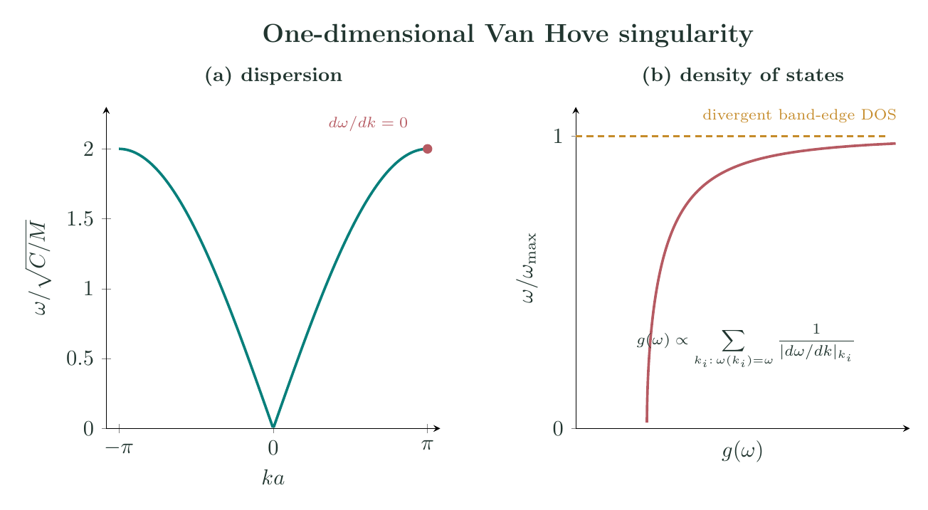
\[\frac{\mathcal N_D(\omega)}{3N} =\left(\frac{\omega}{\omega_D}\right)^3.\]Exact one-dimensional chain density of states
For a monatomic chain of $N$ atoms with nearest-neighbour force constant $K$ and mass $M$,
\[\omega(q)=2\omega_0 \left\lvert\sin\frac{qa}{2}\right\rvert, \qquad \omega_0=\sqrt{\frac KM},\]with $-\pi/a<q\le\pi/a$. For each frequency in $0<\omega<2\omega_0$, there are two wavevectors of opposite sign. Since
\[\sum_q\longrightarrow\frac{Na}{2\pi} \int_{-\pi/a}^{\pi/a}dq,\]the density of states is
\[g(\omega) =\frac{Na}{2\pi} \sum_{q_i} \frac{1}{\left\lvert d\omega/dq\right\rvert_{q_i}}.\]Using
\[\left\lvert\frac{d\omega}{dq}\right\rvert =a\omega_0 \sqrt{1-\left(\frac{\omega}{2\omega_0}\right)^2},\]one obtains
\[\boxed{ g(\omega) =\frac{2N} {\pi\sqrt{4\omega_0^2-\omega^2}}, \qquad 0<\omega<2\omega_0. }\]Its normalization is
\[\int_0^{2\omega_0}g(\omega)\,d\omega=N.\]At the zone boundary, $\omega\to2\omega_0$ and the group velocity tends to zero. Consequently,
\[g(\omega)\sim \frac{N}{\pi\sqrt{\omega_0}}\, \frac{1}{\sqrt{2\omega_0-\omega}},\]which is the inverse-square-root Van Hove singularity of a one-dimensional band maximum.
Van Hove critical points
A Van Hove critical point of branch $s$ occurs at a wavevector $\mathbf q_c$ for which
\[\boxed{ \nabla_{\mathbf q}\omega_{\mathbf q s} \big\rvert_{\mathbf q_c}=0. }\]The constant-frequency-surface formula becomes singular there because its denominator is the group-velocity magnitude. Near an isolated non-degenerate critical point, choose principal axes of the Hessian and write
\[\omega(\mathbf q)-\omega_c \simeq\frac12\sum_{i=1}^{d} \lambda_i k_i^2, \qquad \mathbf k=\mathbf q-\mathbf q_c.\]The signs of the Hessian eigenvalues $\lambda_i$ classify the point:
- all positive: local minimum;
- all negative: local maximum;
- mixed signs: saddle point.
For an extremum in $d$ dimensions, the leading one-sided contribution has the form
\[g_{\mathrm{sing}}(\omega) \propto \left\lvert\omega-\omega_c\right\rvert^{d/2-1} \Theta\!\left[ \pm(\omega-\omega_c) \right],\]where the sign is chosen according to whether the point is a minimum or maximum. Therefore:
- in one dimension, an extremum gives an inverse-square-root divergence;
- in two dimensions, an extremum gives a finite step;
- in three dimensions, an extremum gives a square-root onset or termination.
A two-dimensional saddle point produces a logarithmic divergence,
\[g_{\mathrm{sing}}(\omega) \propto-\ln\left\lvert\omega-\omega_c\right\rvert.\]At a non-degenerate three-dimensional saddle, the density itself is generally finite, but it has a nonanalytic square-root cusp and an infinite one-sided slope in the ideal harmonic limit. The precise regular background and the side on which the cusp appears depend on the Hessian signature and the Brillouin-zone cutoff.
Finite phonon lifetime, isotope disorder, instrumental resolution and anharmonicity broaden ideal singularities into finite peaks or shoulders. The critical-point frequencies remain useful for assigning features in neutron, Raman, infrared and tunnelling spectra.
Thermodynamic use of the density of states
For non-interacting phonons, the vibrational internal energy is
\[U(T)=\int_0^\infty d\omega\, g(\omega)\hbar\omega \left[ \frac{1}{e^{\hbar\omega/(k_{\mathrm B}T)}-1} +\frac12 \right].\]Differentiation gives
\[\boxed{ C_V(T) =k_{\mathrm B}\int_0^\infty d\omega\, g(\omega) \frac{x^2e^x}{(e^x-1)^2}, \qquad x=\frac{\hbar\omega}{k_{\mathrm B}T}. }\]At low temperature only long-wavelength acoustic modes are populated. Since their three-dimensional Debye density varies as $\omega^2$, the integral gives the $T^3$ law. A peak in the density of states is not reproduced one-for-one in heat capacity because the thermal kernel averages a broad range of frequencies.
A species-projected or polarization-projected density of states inserts a weight into the definition:
\[g_\kappa(\omega) =\sum_{\mathbf q s} \left\lvert\mathbf e_\kappa(\mathbf q,s)\right\rvert^2 \delta(\omega-\omega_{\mathbf q s}).\]Such projected densities reveal which atoms participate in a frequency range. A neutron-weighted density additionally contains scattering-length and mass factors and is not, in general, identical to the unweighted phonon density of states.
Worked Debye example
Let
\[n=5.00\times10^{28}\,\mathrm{m^{-3}}, \qquad v_L=6000\,\mathrm{m\,s^{-1}}, \qquad v_T=3200\,\mathrm{m\,s^{-1}}.\]The average velocity is
\[v_D= \left[ \frac13\left( \frac{1}{v_L^3}+\frac{2}{v_T^3} \right) \right]^{-1/3} =3.58\times10^3\,\mathrm{m\,s^{-1}}.\]Therefore
\[q_D=(6\pi^2n)^{1/3} =1.436\times10^{10}\,\mathrm{m^{-1}},\] \[\omega_D=v_Dq_D =5.13\times10^{13}\,\mathrm{rad\,s^{-1}},\] \[f_D=\frac{\omega_D}{2\pi} =8.17\,\mathrm{THz}, \qquad \Theta_D=392\,\mathrm K.\]At $f=2.00\,\mathrm{THz}$,
\[\frac{\mathcal N_D(f)}{3N} =\left(\frac{2.00}{8.17}\right)^3 =1.47\times10^{-2}.\]Only about $1.47\%$ of the Debye acoustic modes lie below this frequency, even though it is about one quarter of the cutoff frequency; the cubic dependence follows from three-dimensional reciprocal-space volume.
Preparation questions
- Define the phonon density of states and prove that its integral is $3rN$ for a crystal with $r$ atoms per primitive cell.
- Derive the constant-frequency-surface expression for $g(\omega)$ and explain why small group velocity enhances the density of states.
- Derive the three-dimensional Debye density of states, including longitudinal and transverse branch counting, and obtain $q_D$, $\omega_D$ and $\Theta_D$.
- Obtain the exact density of states of a nearest-neighbour monatomic chain and identify its Van Hove singularity.
- Classify non-degenerate critical points of a phonon branch using the Hessian of $\omega(\mathbf q)$.
- Compare the singular behaviour at extrema and saddle points in one, two and three dimensions.
- Derive the phonon heat-capacity integral in terms of $g(\omega)$ and explain the low-temperature $T^3$ law.
- For a solid with specified $n$, $v_L$ and $v_T$, calculate its Debye frequency and the fraction of modes below a given frequency.


Discussion