

13 Jul 2026
Hall Effect: Carrier Type, Hall Coefficient, and Carrier Concentration
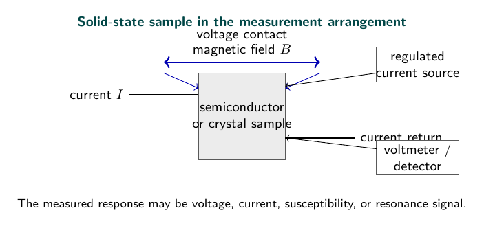
Experimental arrangement
Aim
To determine the Hall coefficient and carrier concentration of a semiconductor sample.
Apparatus
Semiconductor Hall sample, electromagnet, constant-current source, microvoltmeter, Gauss meter, and micrometer.
Theory
An applied longitudinal electric field makes the mobile carriers in a semiconductor acquire a mean drift velocity $v_d$. If a magnetic field $B$ is applied perpendicular to this current, every carrier experiences the transverse Lorentz force $q(\mathbf v_d\times\mathbf B)$. Carriers accumulate at one side of the specimen and leave the opposite side deficient. This charge separation creates a transverse Hall field $E_H$ that grows until
\[qE_H=qv_dB.\]For a rectangular specimen of width $w$ and thickness $t$, $E_H=V_H/w$. The current is $I=nqv_dwt$ for one dominant carrier type. Eliminating $v_d$ gives
\[V_H=\frac{IB}{nqt}.\]The Hall coefficient is therefore
\[R_H=\frac{V_Ht}{IB},\qquad n=\frac{1}{eR_H}.\]For electrons $q=-e$, so $R_H$ is negative; for holes it is positive. The sign of the corrected Hall voltage therefore identifies the majority carrier. A small transverse voltage may exist even at $B=0$ because the contacts are not exactly opposite. Since the true Hall voltage reverses with $I$ or $B$ while the offset does not, reversal readings are combined to remove it.
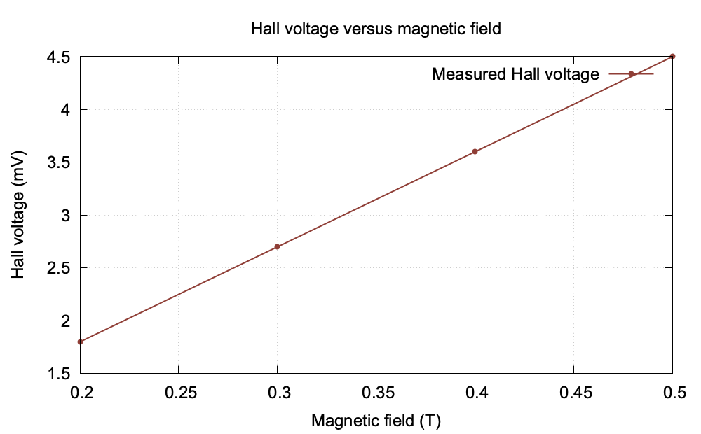
| If the longitudinal conductivity $\sigma$ is also known, the mobility follows from $\mu= | R_H | \sigma$. The Hall angle describes the deflection of current and satisfies $\tan\theta_H=E_H/E_x=\mu B$ in the simple one-carrier model. The linearity of $V_H$ with both $I$ and $B$ is an important experimental check. |
Observations
Sample thickness $t=0.50\,\text{mm}$; current $I=5\,\text{mA}$.
| Magnetic field (T) | Hall voltage (mV) |
|---|---|
| 0.20 | 1.8 |
| 0.30 | 2.7 |
| 0.40 | 3.6 |
| 0.50 | 4.5 |
Graph
Calculation
For $B=0.40\,\text{T}$ and $V_H=3.6\,\text{mV}$,
\[R_H=\frac{3.6\times10^{-3}\times0.50\times10^{-3}}{5\times10^{-3}\times0.40}=9.00\times10^{-4}\,\text{m}^3\text{C}^{-1}.\]Thus
\[n=\frac{1}{eR_H}=\frac{1}{(1.602\times10^{-19})(9.00\times10^{-4})}=6.93\times10^{21}\,\text{m}^{-3}.\]Result
\[\boxed{R_H=9.00\times10^{-4}\,\text{m}^3\text{C}^{-1}},\qquad \boxed{n=6.93\times10^{21}\,\text{m}^{-3}}.\]Precautions
- Reverse the magnetic field and average the Hall readings.
- Keep the sample current constant.
- Ensure that the magnetic field is perpendicular to the current.
Viva Questions
- What is the Hall effect? It is the production of a transverse voltage in a current-carrying sample placed in a magnetic field.
- What determines the sign of Hall voltage? The sign of the dominant charge carriers.
- Why is a thin sample preferred? It gives a measurable Hall voltage for a given current and field.


Discussion