13 Jul 2026

Monte Carlo Simulation of a Two-Dimensional Ising Model

practical ug-vi computational-physics ising-model monte-carlo

Aim

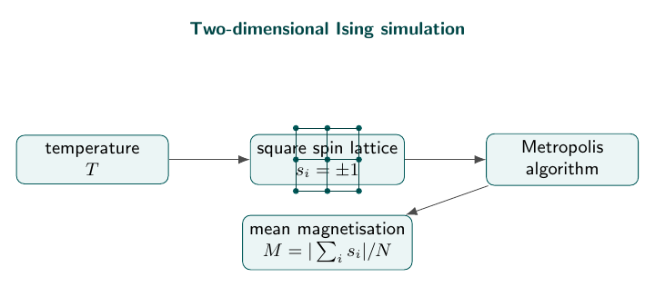
To simulate a two-dimensional Ising model using the Metropolis method and study the variation of magnetisation with temperature.

Apparatus and software

Computer, Maxima or Python, random-number generator, and plotting software.

Figure

Temperature controls the square spin lattice; the Metropolis algorithm produces the mean magnetisation.

Theory

The Ising model represents a lattice of spins $s_i=\pm1$. Neighbouring spins interact through

\[E=-J\sum_{\langle ij\rangle}s_is_j.\]

At temperature $T$, a trial spin reversal with energy change $\Delta E$ is accepted with probability $\min[1,e^{-\Delta E/(k_BT)}]$. Repeating this process generates equilibrium configurations. The magnetisation per spin is

\[M=\frac{1}{N}\left|\sum_i s_i\right|.\]

Observations

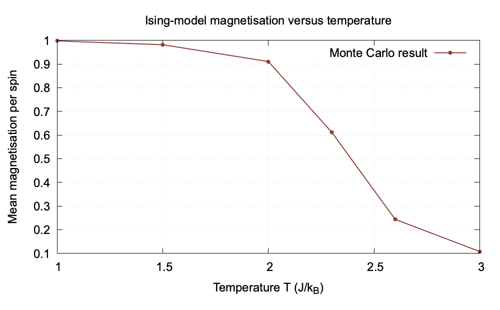
For a $20\times20$ lattice with $J/k_B=1$:

Temperature $T$	Mean magnetisation $M$
1.0	0.998
1.5	0.982
2.0	0.911
2.3	0.612
2.6	0.244
3.0	0.108

Graph

Monte Carlo magnetisation curve for the finite two-dimensional lattice.

Result

The simulation shows an ordered state at low temperature and a disordered state at high temperature, with a sharp reduction in magnetisation near $T\approx2.3J/k_B$ for the finite lattice used.

Viva Questions

1. Why are spins restricted to two values? This is the defining approximation of the Ising model.
2. What is the Metropolis criterion? It gives the probability of accepting an energetically unfavourable trial move.
3. Why are equilibration steps discarded? The initial configuration may not represent thermal equilibrium.

Maxima Code

Download the Maxima calculation file.