

27 Jul 2026
Spherical Harmonics and Their Research Extensions
Spherical harmonics are not merely special functions used to solve the hydrogen atom. They are the natural normal modes of a scalar field on the two-sphere. Their orthogonality, degeneracy, recurrence relations, and coupling rules all follow from the geometry and rotational symmetry of the sphere.
The development below assumes no previous knowledge of spherical harmonics. A scalar field is simply one number assigned to every point: temperature on Earth, pressure on a spherical membrane, or a quantum wave amplitude are examples. A mode is a pattern that keeps its spatial shape while its overall amplitude oscillates. An eigenfunction is the mathematical version of such a mode: an operator acts on it without changing its shape, only multiplying it by a number called the eigenvalue. Spherical harmonics are the angular eigenfunctions selected by a sphere.
The first thirteen sections build the ordinary theory from geometry. The remaining sections then vary the geometry, field, connection, operator, boundary conditions, or dynamics. In this way the reader reaches publication-level research questions by extending a problem whose origin and assumptions are already clear.
This viewpoint is especially useful for research. Once the basic spectral problem is understood, new families of harmonics can be generated by changing one of its ingredients:
\[\boxed{ \text{geometry} + \text{field type} + \text{connection} + \text{operator} + \text{boundary conditions} + \text{dynamics} }\]No finite list can contain every model that might be invented. The classification developed here is more useful: it identifies the independent parts of the spherical-harmonic problem that can be altered, and therefore generates the principal extensions systematically.
1. Why the sphere appears in physics
Consider a problem in three-dimensional space whose physical law is invariant under rotations. Examples include:
- the electrostatic potential outside a localized charge distribution;
- the gravitational field outside a compact body;
- the Schrödinger equation with a central potential;
- acoustic, electromagnetic, elastic, and fluid waves;
- radiation and scattering from localized sources;
- angular correlations measured on a spherical detector.
In Cartesian coordinates the rotational symmetry is hidden among the variables $x$, $y$, and $z$. Spherical coordinates expose it:
\[x=r\sin\theta\cos\phi,\] \[y=r\sin\theta\sin\phi,\] \[z=r\cos\theta,\]with
\[0\leq r<\infty, \qquad 0\leq\theta\leq\pi, \qquad 0\leq\phi<2\pi.\]Here $r$ is distance from the origin, $\theta$ is the polar angle measured downward from the positive $z$ axis, and $\phi$ is the azimuthal angle around that axis. Holding $r$ fixed leaves only $\theta$ and $\phi$, so it restricts the problem to a sphere.
The Euclidean line element becomes
\[ds^2 = dr^2 + r^2d\theta^2 + r^2\sin^2\theta\,d\phi^2.\]At fixed $r$, the remaining geometry is a sphere. The angular area element is
\[d\Omega=\sin\theta\,d\theta\,d\phi.\]The factor $\sin\theta$ is not optional. It is fixed by the geometry and therefore appears in normalization, orthogonality, differential operators, and all angular integrals.
2. Deriving the angular Laplacian
The distance formula determines the differential operator; it is not an independent assumption. On the unit sphere the squared angular distance is
\[d\sigma^2=d\theta^2+\sin^2\theta\,d\phi^2.\]It has metric and inverse metric
\[g_{ab} = \begin{pmatrix} 1&0\\ 0&\sin^2\theta \end{pmatrix}, \qquad g^{ab} = \begin{pmatrix} 1&0\\ 0&1/\sin^2\theta \end{pmatrix},\]and
\[\sqrt{g}=\sqrt{\det g_{ab}}=\sin\theta.\]For any scalar field $f$, the Laplace–Beltrami operator determined by a metric is
\[\Delta f = \frac{1}{\sqrt g} \partial_a \left( \sqrt g\,g^{ab}\partial_b f \right).\]Substitution of the spherical metric gives
\[\boxed{ \Delta_\Omega = \frac{1}{\sin\theta} \frac{\partial}{\partial\theta} \left( \sin\theta\frac{\partial}{\partial\theta} \right) + \frac{1}{\sin^2\theta} \frac{\partial^2}{\partial\phi^2} }\]This calculation explains at once why the factor $\sin\theta$ occurs in both the area element and the angular differential operator.
The full scalar Laplacian in spherical coordinates is
\[\nabla^2 = \frac{1}{r^2} \frac{\partial}{\partial r} \left( r^2\frac{\partial}{\partial r} \right) + \frac{1}{r^2}\Delta_\Omega,\]where $\Delta_\Omega$ is precisely the unit-sphere operator just derived.
A simple wave field $u$ obeys
\[\frac{\partial^2u}{\partial t^2} = v^2\nabla^2u,\]where $v$ is the wave speed. For a single-frequency oscillation
\[u(\boldsymbol r,t) = \operatorname{Re} \left[ \Psi(\boldsymbol r)e^{-\mathrm i\omega t} \right],\]the wave equation reduces to the Helmholtz equation
\[\nabla^2\Psi+k^2\Psi=0.\]Here $k=\omega/v$. Thus the eigenvalue problem below already describes ordinary classical waves; quantum mechanics is an additional application, not a prerequisite.
Write
\[\Psi(r,\theta,\phi) = R(r)Y(\theta,\phi).\]After substitution and division by $RY$, the radial variables and angular variables occur in two terms whose sum is zero. Because $r$ can be changed without changing $\theta$ or $\phi$, each term must equal a constant. Calling the angular constant $\lambda$, the angular equation can be written
\[\boxed{ -\Delta_\Omega Y=\lambda Y }\]Spherical harmonics are therefore eigenfunctions of the intrinsic Laplacian of the sphere.
The same angular equation follows from the Schrödinger equation
\[\left[ -\frac{\hbar^2}{2\mu}\nabla^2+V(r) \right]\Psi = E\Psi\]for every central potential $V(r)$. The radial physics changes from one central potential to another, but the angular eigenfunctions remain spherical harmonics.
3. Separation of the angular equation
Let
\[Y(\theta,\phi) = \Theta(\theta)\Phi(\phi).\]Substitution in $-\Delta_\Omega Y=\lambda Y$, division by $\Theta\Phi$, and multiplication by $\sin^2\theta$ gives
\[-\frac{\sin\theta}{\Theta} \frac{d}{d\theta} \left( \sin\theta\frac{d\Theta}{d\theta} \right) - \frac{1}{\Phi}\frac{d^2\Phi}{d\phi^2} = \lambda\sin^2\theta.\]The only $\phi$-dependent term must be a constant. Write that constant as $m^2$. The azimuthal equation is then
\[\frac{d^2\Phi}{d\phi^2} + m^2\Phi=0.\]Its solutions are
\[\Phi(\phi)=e^{\mathrm i m\phi}.\]A scalar field must be single-valued:
\[\Phi(\phi+2\pi)=\Phi(\phi).\]Hence,
\[m\in\mathbb Z.\]The polar equation is
\[\frac{1}{\sin\theta} \frac{d}{d\theta} \left( \sin\theta\frac{d\Theta}{d\theta} \right) + \left[ \lambda - \frac{m^2}{\sin^2\theta} \right]\Theta =0.\]Set
\[x=\cos\theta.\]Then
\[\boxed{ (1-x^2)\frac{d^2\Theta}{dx^2} - 2x\frac{d\Theta}{dx} + \left[ \lambda-\frac{m^2}{1-x^2} \right]\Theta =0 }\]This is the associated Legendre equation.
4. Why the quantum numbers are discrete
The north and south poles correspond to
\[x=1 \qquad\text{and}\qquad x=-1.\]Generic solutions of the associated Legendre equation diverge at one or both endpoints. Requiring the field to remain finite and square-integrable on the complete sphere quantizes the separation constant:
\[\lambda=\ell(\ell+1),\]where
\[\ell=0,1,2,\ldots\]and
\[-\ell\leq m\leq\ell.\]Thus, the discrete angular spectrum is not inserted by hand. It follows from global regularity and single-valuedness on a compact manifold.
The regular polar solutions are the associated Legendre functions
\[P_\ell^m(\cos\theta).\]5. Normalized spherical harmonics
Let the associated Legendre function $P_\ell^m$ include the Condon–Shortley phase. The normalized spherical harmonic is then
\[\boxed{ Y_\ell^m(\theta,\phi) = \sqrt{ \frac{2\ell+1}{4\pi} \frac{(\ell-m)!}{(\ell+m)!} } P_\ell^m(\cos\theta) e^{\mathrm i m\phi} }\]If $P_\ell^m$ is instead defined without the Condon–Shortley phase, an external factor $(-1)^m$ must multiply this formula. A calculation must use one convention consistently, especially when comparing ladder operators, Clebsch–Gordan coefficients, and software output.
Negative-$m$ harmonics satisfy
\[Y_\ell^{-m} = (-1)^m \left(Y_\ell^m\right)^*.\]The lowest harmonics are
\[Y_0^0=\frac{1}{\sqrt{4\pi}},\] \[Y_1^0 = \sqrt{\frac{3}{4\pi}}\cos\theta,\] \[Y_1^{\pm1} = \mp \sqrt{\frac{3}{8\pi}} \sin\theta\,e^{\pm\mathrm i\phi},\]and
\[Y_2^0 = \sqrt{\frac{5}{16\pi}} \left(3\cos^2\theta-1\right).\]6. Orthogonality and completeness
The natural inner product on the sphere is
\[\langle f,g\rangle = \int_0^{2\pi} \int_0^\pi f^*(\theta,\phi) g(\theta,\phi) \sin\theta\,d\theta\,d\phi.\]Spherical harmonics are orthonormal:
\[\boxed{ \int \left(Y_\ell^m\right)^* Y_{\ell'}^{m'} \,d\Omega = \delta_{\ell\ell'}\delta_{mm'} }\]They are also complete in the space of square-integrable scalar functions on the sphere:
\[f(\theta,\phi) = \sum_{\ell=0}^{\infty} \sum_{m=-\ell}^{\ell} a_{\ell m}Y_\ell^m(\theta,\phi),\]where
\[a_{\ell m} = \int \left(Y_\ell^m\right)^* f\,d\Omega.\]Completeness can be expressed as a spherical delta function:
\[\sum_{\ell=0}^{\infty} \sum_{m=-\ell}^{\ell} Y_\ell^m(\Omega) \left(Y_\ell^m(\Omega')\right)^* = \delta(\Omega-\Omega').\]This is why spherical harmonics can reconstruct an arbitrary sufficiently regular angular field.
7. Angular momentum from geometry
In quantum mechanics,
\[\hat L^2=-\hbar^2\Delta_\Omega,\]and
\[\hat L_z = -\mathrm i\hbar \frac{\partial}{\partial\phi}.\]Therefore,
\[\boxed{ \hat L^2Y_\ell^m = \hbar^2\ell(\ell+1)Y_\ell^m }\]and
\[\boxed{ \hat L_zY_\ell^m = \hbar mY_\ell^m }\]The $2\ell+1$ values of $m$ form one irreducible angular-momentum multiplet. Rotational symmetry makes them degenerate whenever the Hamiltonian depends only on $r$ and $\hat L^2$.
The ladder operators are
\[\hat L_\pm = \hbar e^{\pm\mathrm i\phi} \left( \pm\frac{\partial}{\partial\theta} + \mathrm i\cot\theta \frac{\partial}{\partial\phi} \right).\]They act as
\[\boxed{ \hat L_\pm Y_\ell^m = \hbar \sqrt{ (\ell\mp m)(\ell\pm m+1) } Y_\ell^{m\pm1} }\]The ladder action changes $m$ without changing $\ell$. It constructs the complete multiplet from a highest- or lowest-weight state.
8. Parity, phase winding, and nodes
Under spatial inversion,
\[(\theta,\phi) \longmapsto (\pi-\theta,\phi+\pi).\]Spherical harmonics have definite parity:
\[\boxed{ Y_\ell^m(-\hat{\boldsymbol r}) = (-1)^\ell Y_\ell^m(\hat{\boldsymbol r}) }\]For complex harmonics, the factor $e^{\mathrm i m\phi}$ has phase winding $m$ around the polar axis. Its modulus is independent of $\phi$, so the complex harmonic does not have the meridional sign-changing planes seen in the usual real orbital pictures.
Real tesseral harmonics are obtained from
\[Y_{\ell m}^{(c)} = \sqrt2\,\operatorname{Re}Y_\ell^m,\]and
\[Y_{\ell m}^{(s)} = \sqrt2\,\operatorname{Im}Y_\ell^m\]for $m>0$. These real combinations have $\lvert m\rvert$ nodal planes through the polar axis and $\ell-\lvert m\rvert$ polar nodes arising from the associated Legendre factor.
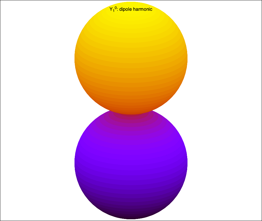
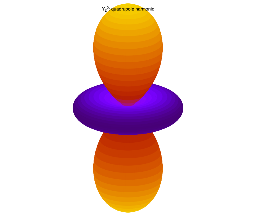
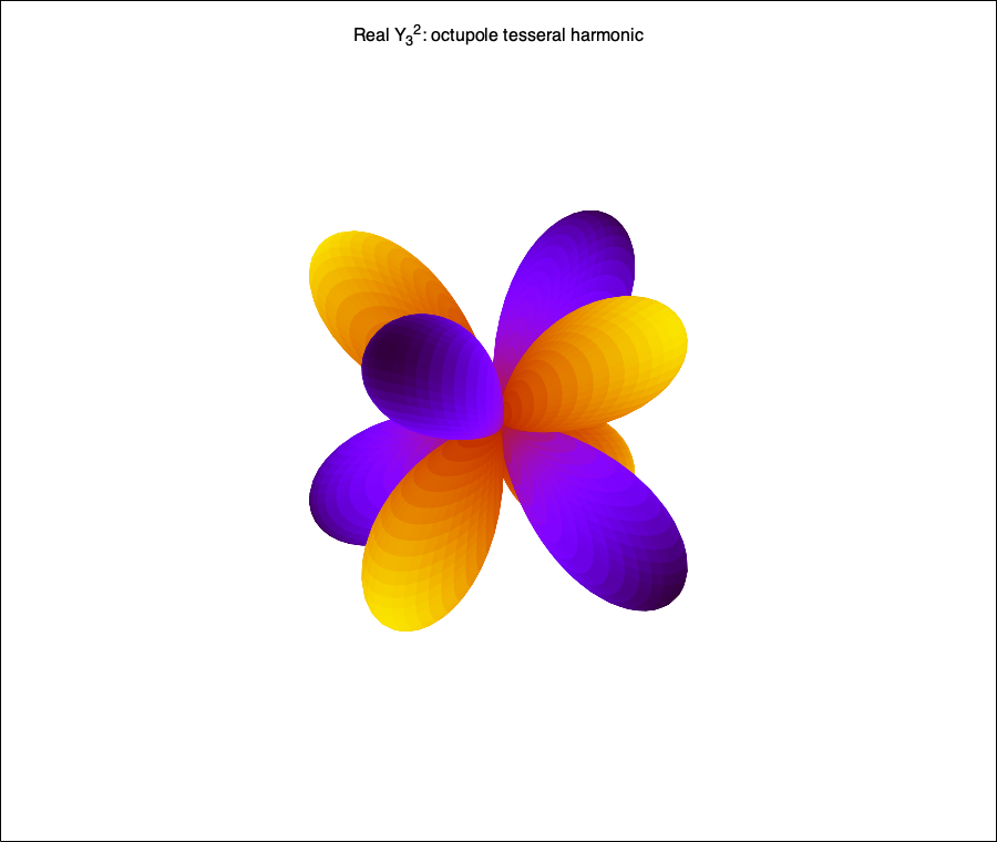
9. Maxima-generated three-dimensional harmonics
The following surfaces were generated directly by the Maxima file linked at the end of this post. The plotted radius is
\[r(\theta,\phi)=\left\lvert Y(\theta,\phi)\right\rvert,\]while the surface colour records the sign of the corresponding real angular amplitude. The colour change therefore retains sign information that the absolute magnitude alone would lose.
10. Rotations and Wigner matrices
A rotation does not mix different values of $\ell$. It mixes only the $2\ell+1$ functions within one multiplet:
\[Y_\ell^m(R^{-1}\Omega) = \sum_{m'=-\ell}^{\ell} D_{m'm}^{(\ell)}(R) Y_\ell^{m'}(\Omega).\]The matrices
\[D^{(\ell)}(R)\]form the irreducible representations of the rotation group. This statement is deeper than a coordinate transformation: it explains why a fixed $\ell$ sector is the natural unit for rotationally covariant calculations.
The sphere may be viewed as the homogeneous space
\[S^2\simeq SO(3)/SO(2).\]Scalar spherical harmonics are therefore examples of harmonic analysis on a group quotient. Wigner $D$-functions provide the parent construction on $SO(3)$ itself.
11. The addition theorem
Let $\gamma$ be the angle between two unit vectors:
\[\cos\gamma = \hat{\boldsymbol r}\cdot\hat{\boldsymbol r}'.\]Rotational invariance implies that summing over a complete $m$ multiplet can depend only on $\gamma$. The result is
\[\boxed{ \sum_{m=-\ell}^{\ell} Y_\ell^m(\Omega) \left(Y_\ell^m(\Omega')\right)^* = \frac{2\ell+1}{4\pi} P_\ell(\cos\gamma) }\]This theorem converts an orientation-dependent sum into a single Legendre polynomial. It underlies rotationally invariant kernels, angular power spectra, Green functions, and multipole expansions.
For example,
\[\frac{1}{\lvert\boldsymbol r-\boldsymbol r'\rvert} = 4\pi \sum_{\ell=0}^{\infty} \sum_{m=-\ell}^{\ell} \frac{1}{2\ell+1} \frac{r_<^\ell}{r_>^{\ell+1}} Y_\ell^m(\Omega) \left(Y_\ell^m(\Omega')\right)^*,\]where
\[r_<=\min(r,r'), \qquad r_>=\max(r,r').\]This is the basic bridge from spherical harmonics to electrostatic, gravitational, and scattering multipoles.
12. The supplied recurrence relation
The associated Legendre recurrence is
\[(2\ell+1)xP_\ell^m(x) = (\ell-m+1)P_{\ell+1}^m(x) + (\ell+m)P_{\ell-1}^m(x).\]Set
\[x=\cos\theta\]and write
\[Y_\ell^m = N_{\ell m}P_\ell^m(\cos\theta)e^{\mathrm i m\phi},\]where
\[N_{\ell m} = \sqrt{ \frac{2\ell+1}{4\pi} \frac{(\ell-m)!}{(\ell+m)!} }.\]After multiplication by $N_{\ell m}e^{\mathrm i m\phi}$, the coefficient of $Y_{\ell+1}^m$ is
\[\frac{\ell-m+1}{2\ell+1} \frac{N_{\ell m}}{N_{\ell+1,m}} = \sqrt{ \frac{(\ell+1)^2-m^2} {(2\ell+1)(2\ell+3)} },\]and the coefficient of $Y_{\ell-1}^m$ is
\[\frac{\ell+m}{2\ell+1} \frac{N_{\ell m}}{N_{\ell-1,m}} = \sqrt{ \frac{\ell^2-m^2} {(2\ell-1)(2\ell+1)} }.\]Therefore,
\[\boxed{ \begin{aligned} \cos\theta\,Y_\ell^m ={}& \sqrt{ \frac{(\ell+1)^2-m^2} {(2\ell+1)(2\ell+3)} } Y_{\ell+1}^m \\[4pt] &+ \sqrt{ \frac{\ell^2-m^2} {(2\ell-1)(2\ell+1)} } Y_{\ell-1}^m. \end{aligned} }\]This is the recurrence shown in the supplied expression, with
\[J\longleftrightarrow\ell, \qquad M\longleftrightarrow m.\]Its importance is physical as well as computational. It gives the matrix element
\[\begin{aligned} \left\langle\ell'm'\right\rvert \cos\theta \left\lvert\ell m\right\rangle ={}& \delta_{m'm} \sqrt{ \frac{(\ell+1)^2-m^2} {(2\ell+1)(2\ell+3)} } \delta_{\ell',\ell+1} \\[4pt] &+ \delta_{m'm} \sqrt{ \frac{\ell^2-m^2} {(2\ell-1)(2\ell+1)} } \delta_{\ell',\ell-1}. \end{aligned}\]Therefore an axial dipole factor obeys the selection rules
\[\boxed{ \Delta\ell=\pm1, \qquad \Delta m=0. }\]Repeated use gives sparse representations of powers of $\cos\theta$. For example, $\cos^2\theta$ connects
\[\Delta\ell=0,\pm2.\]This sparse algebra is useful in Stark problems, aligned rotors, anisotropic traps, molecular orientation, angular quenches, and numerical spectral matrices.
13. Products, Gaunt coefficients, and selection rules
The product of two spherical harmonics can be expanded into spherical harmonics:
\[Y_{\ell_1}^{m_1}Y_{\ell_2}^{m_2} = \sum_{LM} C_{\ell_1m_1,\ell_2m_2}^{LM} Y_L^M.\]The allowed values follow from angular-momentum addition:
\[\lvert\ell_1-\ell_2\rvert \leq L \leq \ell_1+\ell_2,\]and
\[M=m_1+m_2.\]The integral of three harmonics is the Gaunt coefficient:
\[\begin{aligned} \int Y_{\ell_1}^{m_1} Y_{\ell_2}^{m_2} Y_{\ell_3}^{m_3} \,d\Omega ={}& \sqrt{ \frac{ (2\ell_1+1)(2\ell_2+1)(2\ell_3+1) }{4\pi} } \\ &\times \begin{pmatrix} \ell_1&\ell_2&\ell_3\\ 0&0&0 \end{pmatrix} \begin{pmatrix} \ell_1&\ell_2&\ell_3\\ m_1&m_2&m_3 \end{pmatrix}. \end{aligned}\]It vanishes unless:
\[m_1+m_2+m_3=0,\]the three $\ell$ values satisfy the triangle condition, and
\[\ell_1+\ell_2+\ell_3\]has even parity.
These are not merely integration shortcuts. They determine which nonlinear mode couplings, transition amplitudes, and perturbative corrections are forbidden before any radial calculation is attempted.
14. A master formulation for extensions
The scalar spherical-harmonic problem can be generalized to
\[\boxed{ \mathcal L[g,\nabla^{(A)},s,V,\mathcal B] \Psi = \lambda\,w\,\Psi. }\]Here:
- $g$ specifies the geometry;
- $\nabla^{(A)}$ specifies an ordinary or gauge-covariant connection;
- $s$ specifies scalar, spinor, vector, or tensor character;
- $V$ specifies additional angular interactions;
- $\mathcal B$ specifies global regularity or boundary conditions;
- $w$ specifies the inner-product weight.
Ordinary spherical harmonics correspond to the unit-sphere metric, a scalar field, no gauge connection, no additional potential, and global regularity. The main research extensions arise by changing one or more entries in this operator.
15. Extension by changing the field representation
15.1 Real and point-group-adapted harmonics
Real tesseral harmonics replace complex phases by sine and cosine combinations. Further linear combinations can be adapted to a discrete point group, producing cubic, tetrahedral, or icosahedral harmonics.
The continuous $SO(3)$ multiplet then decomposes into irreducible representations of the smaller symmetry group. This is useful for crystal fields, molecular orbitals, ligand environments, anisotropic nanoparticles, and symmetry-breaking perturbations.
15.2 Spin-weighted spherical harmonics
A field whose local phase changes under rotation of the tangent-frame basis has spin weight $s$. Its natural basis is
\[{}_sY_\ell^m.\]Spin-raising and spin-lowering operators satisfy, in a common convention,
\[\eth\,{}_sY_\ell^m = \sqrt{(\ell-s)(\ell+s+1)} \,{}_{s+1}Y_\ell^m,\] \[\bar\eth\,{}_sY_\ell^m = - \sqrt{(\ell+s)(\ell-s+1)} \,{}_{s-1}Y_\ell^m.\]They are required for polarization, helicity fields, gravitational waves, and tangent-plane tensor data.
15.3 Vector spherical harmonics
A vector field needs three angular directions. A standard basis is
\[\boldsymbol Y_{\ell m} = Y_\ell^m\hat{\boldsymbol r},\] \[\boldsymbol\Psi_{\ell m} = \frac{r\nabla Y_\ell^m} {\sqrt{\ell(\ell+1)}},\] \[\boldsymbol\Phi_{\ell m} = \hat{\boldsymbol r} \times \boldsymbol\Psi_{\ell m}.\]These separate radial, electric-type, and magnetic-type components. They are natural for Maxwell fields, elastic waves, fluid velocity fields, magnetic multipoles, and vector scattering.
15.4 Tensor and spinor spherical harmonics
Tensor harmonics separate trace, longitudinal, transverse, electric-parity, and magnetic-parity sectors of tensor fields. Spinor spherical harmonics couple orbital angular momentum to spin one-half:
\[\mathcal Y_{j\ell m_j} = \sum_{m,m_s} \langle\ell m,\tfrac12m_s\mid jm_j\rangle Y_\ell^m\chi_{m_s}.\]These bases are required for Dirac central-force problems, relativistic atoms, curved-space fields, gravitational perturbations, and tensor tomography.
16. Extension by changing the geometry
16.1 Spheroidal harmonics
Separation in oblate or prolate spheroidal geometry gives
\[\frac{1}{\sin\theta} \frac{d}{d\theta} \left( \sin\theta\frac{dS}{d\theta} \right) + \left[ \lambda + c^2\cos^2\theta - \frac{m^2}{\sin^2\theta} \right]S =0.\]As
\[c\to0,\]the spheroidal harmonics reduce to spherical harmonics. Finite $c$ mixes spherical modes with the same $m$ and parity. Perturbation theory, continued fractions, recurrence stability, and large-$c$ asymptotics all provide research directions.
16.2 Hyperspherical harmonics
On the sphere $S^{d-1}$,
\[-\Delta_{S^{d-1}}Y_{\ell,\boldsymbol\mu} = \ell(\ell+d-2)Y_{\ell,\boldsymbol\mu}.\]The degeneracy is
\[g_\ell^{(d)} = \frac{ (2\ell+d-2)(\ell+d-3)! }{ \ell!(d-2)! }.\]Hyperspherical harmonics are useful for few-body quantum mechanics, higher-dimensional gravity, multidimensional scattering, and collective coordinates.
16.3 Perturbed spheres and spectral geometry
For
\[g_{ab} = g_{ab}^{(0)} + \varepsilon h_{ab},\]the Laplace–Beltrami operator becomes
\[\Delta_g = \Delta_\Omega + \varepsilon\,\delta\Delta + O(\varepsilon^2).\]The perturbation splits the $m$ degeneracy and couples different $\ell$ sectors. The coupling matrix is determined by harmonic overlaps of the geometric deformation. This provides a systematic theory for nearly spherical resonators, droplets, shells, cells, planets, and nanostructures.
16.4 Caps, punctures, cones, and interfaces
If the domain is only part of a sphere, regularity at both poles is replaced by boundary or interface conditions. The spectrum need not be $\ell(\ell+1)$, degeneracies split, and edge-localized angular modes may appear.
The essential research question becomes the relation among geometry, boundary conditions, self-adjointness, and spectral flow.
17. Extension by adding gauge structure and topology
For a charged field on a sphere with a magnetic monopole, ordinary derivatives are replaced by covariant derivatives:
\[\boldsymbol D = \boldsymbol\nabla - \frac{\mathrm i q}{\hbar}\boldsymbol A.\]The resulting eigenfunctions are monopole harmonics. They are not globally represented by one nonsingular vector potential; different gauge patches must be related by transition functions.
The monopole charge shifts the allowed lowest angular momentum and introduces topological information. Research extensions include:
- Berry connections and geometric phases;
- Chern numbers and flux quantization;
- Landau levels on curved surfaces;
- gauge-covariant spin and vector harmonics;
- monopole harmonics on deformed or non-Hermitian spheres.
Here topology is part of the eigenfunction space itself, not merely an added potential.
18. Extension by changing the operator
18.1 Rational and Darboux extensions
For fixed $m$, the polar operator is a Sturm–Liouville operator:
\[\mathcal L_m = - \frac{1}{\sin\theta} \frac{d}{d\theta} \left( \sin\theta\frac{d}{d\theta} \right) + \frac{m^2}{\sin^2\theta}.\]A Darboux factorization introduces an intertwining operator $\mathcal A$ such that
\[\mathcal A\mathcal L_m = \widetilde{\mathcal L}_m\mathcal A.\]The transformed operator may contain a rational angular potential and have eigenfunctions built from exceptional Jacobi or associated-Legendre-type systems.
A publication-level construction must establish:
- regularity of the rational terms on the physical interval;
- the correct positive weight and operator domain;
- missing, added, or isospectral states;
- completeness of the exceptional basis;
- modified recurrence and coupling rules;
- observable consequences beyond a change of notation.
This route connects spherical harmonics directly to supersymmetric quantum mechanics, exceptional orthogonal polynomials, rational oscillators, and angular quench models.
18.2 Non-Hermitian and symmetry-constrained angular operators
An angular potential may be complex:
\[\mathcal L = -\Delta_\Omega + V_{\mathrm R}(\theta,\phi) + \mathrm iV_{\mathrm I}(\theta,\phi).\]Right and left eigenfunctions then differ:
\[\mathcal L\Psi_n^{\mathrm R} = \lambda_n\Psi_n^{\mathrm R},\] \[\mathcal L^\dagger\Psi_n^{\mathrm L} = \lambda_n^*\Psi_n^{\mathrm L}.\]Orthogonality is replaced by biorthogonality. Exceptional points, complex spectral transitions, nonorthogonality enhancement, and generalized selection rules become possible.
18.3 Fractional and nonlocal angular operators
Spectral calculus defines
\[(-\Delta_\Omega)^\alpha Y_\ell^m = [\ell(\ell+1)]^\alpha Y_\ell^m.\]This produces fractional diffusion and nonlocal dynamics on a sphere without abandoning the harmonic basis. More general integral kernels can mix $\ell$ sectors while preserving or breaking rotational invariance.
18.4 Matrix-valued and coupled-channel harmonics
Internal spin, band, polarization, or component indices turn the angular operator into a matrix:
\[\sum_b \mathcal L_{ab}\Psi_b = \lambda\Psi_a.\]The problem combines angular selection rules with avoided crossings, topological band structure, channel conversion, and non-Abelian gauge connections.
19. Deformed symmetry and noncommutative spheres
19.1 Fuzzy-sphere harmonics
On a fuzzy sphere, coordinates become matrices:
\[[X_i,X_j] = \mathrm i\lambda\epsilon_{ijk}X_k.\]Functions are replaced by matrices, and spherical harmonics become irreducible tensor operators. For an $N$-dimensional representation, the angular expansion terminates at finite $\ell$.
This gives a symmetry-preserving ultraviolet cutoff and connects angular spectra to noncommutative geometry, matrix models, finite quantum systems, and regularized field theories.
19.2 Quantum-group and (q)-deformed harmonics
Replacing $SO(3)$ or $SU(2)$ by a quantum group deforms ladder coefficients, Clebsch–Gordan rules, and addition theorems. The ordinary theory is recovered as
\[q\to1.\]The meaningful physical question is which observable or geometry requires the deformation, rather than merely replacing integers by $q$-numbers.
19.3 Superspherical harmonics
If bosonic angular coordinates are supplemented by fermionic coordinates, the relevant symmetry becomes a supergroup and the harmonics live on a supersphere. Such constructions extend multiplets, degeneracies, and orthogonality to graded spaces.
20. Dynamic and nonlinear extensions
For a time-dependent field,
\[\Psi(\Omega,t) = \sum_{\ell m} a_{\ell m}(t)Y_\ell^m(\Omega).\]A rotationally invariant linear operator evolves each $\ell,m$ independently. An anisotropic perturbation produces a coupling matrix:
\[\mathrm i\dot a_{\ell m} = \sum_{\ell'm'} H_{\ell m,\ell'm'}(t) a_{\ell'm'}.\]Nonlinear terms generate products of harmonics. Gaunt coefficients and higher Wigner symbols then determine the mode-coupling network.
This framework supports research on:
- nonlinear waves and turbulence on spherical surfaces;
- rotating condensates and angular quenches;
- parametric resonance and Floquet angular modes;
- synchronization between angular sectors;
- open-system angular decoherence;
- entanglement and information flow among multipoles.
The selection rules identify the allowed network before time propagation is performed.
21. Statistical, inverse, and computational extensions
For a random scalar field with coefficients $a_{\ell m}$, rotationally invariant second-order information is summarized by
\[C_\ell = \frac{1}{2\ell+1} \sum_{m=-\ell}^{\ell} \left\langle \lvert a_{\ell m}\rvert^2 \right\rangle.\]This angular power spectrum is complete only for a Gaussian random field. Non-Gaussian information requires higher correlations such as the bispectrum and trispectrum, whose selection rules are controlled by $3j$, $6j$, and higher angular-momentum symbols.
This mirrors the covariance lesson for continuous-variable quantum states: second-order spectra completely determine Gaussian statistics but not general statistics.
Inverse problems attempt to reconstruct sources, shapes, potentials, or material parameters from measured multipoles. Their central issues are:
- incomplete angular coverage;
- noise and regularization;
- finite band limits;
- stability of high-$\ell$ reconstruction;
- symmetry-induced nonuniqueness.
At large $\ell$, direct factorial formulas become numerically unstable. Stable recurrences, logarithmic normalization, Gauss–Legendre quadrature, fast Fourier transforms in $\phi$, and controlled truncation errors are part of the mathematical physics, not merely programming details.
22. Rotation-equivariant computation and learning
An $SO(3)$-equivariant algorithm must transform multipole coefficients within the correct $\ell$ representation. Tensor products are reduced with Clebsch–Gordan coefficients:
\[(\ell_1)\otimes(\ell_2) = \bigoplus_{L=\lvert\ell_1-\ell_2\rvert}^{\ell_1+\ell_2} (L).\]This is the foundation of rotation-equivariant numerical architectures and data-driven models. A research problem becomes physically meaningful when the equivariance is connected to conservation laws, reduced sample complexity, interpretable multipoles, or controlled approximation error.
23. A systematic map of research directions
The extensions can be organized by the ingredient changed:
| Changed ingredient | Representative extensions | Central research question |
|---|---|---|
| Field representation | real, spin-weighted, vector, tensor, spinor | How do spin and polarization modify spectra and selection rules? |
| Geometry | spheroid, hypersphere, perturbed sphere, cap | How do curvature and boundaries split or localize modes? |
| Gauge connection | monopole, Berry, non-Abelian connection | How does topology modify allowed multiplets and phases? |
| Angular operator | rational, fractional, matrix, non-Hermitian | Which spectral and completeness properties survive? |
| Symmetry algebra | point group, fuzzy sphere, quantum group, supergroup | How are multiplets, products, and degeneracies deformed? |
| Dynamics | driven, open, nonlinear, Floquet | Which angular channels exchange energy or information? |
| Statistics | power spectrum, bispectrum, random fields | Which correlations lie beyond second-order information? |
| Computation | fast transforms, sparse recurrences, equivariant models | How can high-order modes be calculated stably and verifiably? |
This table is generative. A new model may combine several rows—for example, a spin-weighted, non-Hermitian spheroidal operator with a gauge connection.
24. How an extension becomes a research publication
A useful extension requires more than writing a modified differential equation. Its scientific content normally has five connected layers.
First, the operator and its domain must be defined precisely. This includes the metric, measure, boundary conditions, singular points, and adjoint.
Second, the spectral structure must be established: eigenvalues, degeneracies, orthogonality or biorthogonality, completeness, and limiting cases.
Third, the analytic mechanism should be identified. It may be a recurrence, intertwiner, perturbation series, representation, selection rule, or asymptotic regime.
Fourth, symbolic and numerical results must be independently verifiable. Residuals, normalization, convergence with angular cutoff, and symmetry constraints provide stronger evidence than plots alone.
Finally, the extension should change a physical prediction or mathematical capability: a spectrum, transition amplitude, scattering coefficient, topological invariant, localization measure, information quantity, or computational scaling.
25. Research problems naturally suggested by this framework
Several problem families follow directly from combining the preceding extensions.
Exceptional angular harmonics
Construct globally regular Darboux extensions of the associated Legendre operator, determine their positive weight and completeness, derive their finite- or higher-term recurrence relations, and calculate how their Gaunt coefficients differ from the ordinary selection rules.
Non-Hermitian spheroidal harmonics
Track exceptional points as the spheroidal parameter and gain–loss profile vary. Determine biorthogonal normalization, phase rigidity, spectral sensitivity, and the effect on partial-wave scattering.
Gauge-covariant exceptional harmonics
Combine monopole topology with a rational angular deformation. The main challenge is compatibility among gauge patches, regularity, flux quantization, and the Darboux transformation.
Perturbed-sphere mode coupling
Derive the mode-coupling matrix generated by a controlled geometric deformation. Compare perturbation theory with a direct numerical Laplace–Beltrami spectrum and identify symmetry-protected crossings.
Non-Gaussian angular information
Treat multipole amplitudes as quantum or stochastic modes. Compare the information contained in $C_\ell$ with exact higher-order or reduced-state measures after an anisotropic quench.
Fuzzy-sphere continuum convergence
Quantify how finite matrix harmonics reproduce continuum spectra, products, and correlation functions as the matrix dimension increases. Establish error bounds rather than relying only on visual convergence.
Each family has an exact ordinary-spherical limit, a controllable deformation parameter, and measurable quantities suitable for analytic and computational cross-checks.
26. Central conclusion
Spherical harmonics are the scalar spectral basis selected by the metric, topology, and rotation group of the two-sphere:
\[\boxed{ -\Delta_\Omega Y_\ell^m = \ell(\ell+1)Y_\ell^m. }\]Their recurrences, ladder operations, addition theorem, and coupling coefficients are different expressions of the same rotational structure.
Research extensions become systematic when one asks which ingredient of the base problem has changed. Geometry leads to spheroidal, hyperspherical, and perturbed-sphere modes. Field character leads to spin, vector, tensor, and spinor harmonics. Connections lead to monopole and topological harmonics. Modified operators lead to rational, fractional, coupled, and non-Hermitian systems. Deformed symmetry leads to point-group, fuzzy, quantum-group, and superspherical bases. Dynamics and statistics turn the static basis into a network of coupled angular modes.
27. Maxima file for calculation and three-dimensional plotting
The accompanying Maxima file verifies a Laplace–Beltrami eigenvalue, normalization, a ladder operation, the supplied $\cos\theta$ recurrence, and a Gaunt coefficient. It also generates the three 3D illustrations used above.
After downloading it, open a terminal in the folder containing the file and run:
maxima --batch=spherical-harmonics-research.mac
The three PNG illustrations will be written into the same working folder.
Download the complete Maxima calculation and 3D plotting file


Discussion