D’Alembert’s Principle, Lagrange’s Equation and Its Simple Applications
1. D’Alembert’s Principle
D’Alembert’s principle is a fundamental concept in classical mechanics that provides an alternative formulation of Newton’s second law by incorporating the concept of virtual work. It states that the sum of the differences between the applied forces and the inertial forces (also called the generalized forces) acting on a system in equilibrium is zero when projected along any virtual displacement.
1.1 Mathematical Formulation
Consider a system of \(N\) particles, where each particle has mass \(m_i\), position vector \(\mathbf{r}_i\), and is subject to an external force \(\mathbf{F}_i\). Newton’s second law states:
\[m_i \ddot{\mathbf{r}}_i = \mathbf{F}_i\]D’Alembert’s principle introduces the concept of inertial force:
\[\mathbf{F}_i - m_i \ddot{\mathbf{r}}_i = 0\]For an infinitesimal virtual displacement \(\delta \mathbf{r}_i\), the principle states:
\[\sum_{i=1}^{N} (\mathbf{F}_i - m_i \ddot{\mathbf{r}}_i) \cdot \delta \mathbf{r}_i = 0\]Since the constraint forces do no virtual work (ideal constraints), we are left with only generalized forces:
\[\sum_{i=1}^{N} (\mathbf{F}_i^{(a)} - m_i \ddot{\mathbf{r}}_i) \cdot \delta \mathbf{r}_i = 0\]where \(\mathbf{F}_i^{(a)}\) represents the applied forces excluding constraint forces.
2. Lagrange’s Equation
Lagrange’s equation is derived using D’Alembert’s principle and is particularly useful in dealing with systems having constraints.
2.1 Generalized Coordinates
A system with \(N\) particles and \(k\) constraint equations can be described using a reduced set of generalized coordinates:
\[q_1, q_2, \dots, q_n, \quad n = 3N - k\]The relationship between Cartesian coordinates and generalized coordinates is given by:
\[\mathbf{r}_i = \mathbf{r}_i(q_1, q_2, ..., q_n, t)\]The virtual displacement then transforms as:
\[\delta \mathbf{r}_i = \sum_{j=1}^{n} \frac{\partial \mathbf{r}_i}{\partial q_j} \delta q_j\]Using these transformations, D’Alembert’s principle can be rewritten in terms of generalized coordinates.
2.2 Derivation of Lagrange’s Equation
3. Simple Applications of Lagrange’s Equations
3.1 Simple Pendulum
A simple pendulum consists of a mass \(m\) attached to a string of length \(l\). The generalized coordinate is the angular displacement \(\theta\).
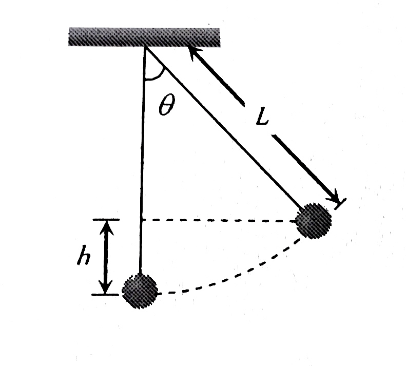
🔹 Coordinates
Use angle \(\theta\) as generalized coordinate.
- Position: \(x = \ell \sin \theta, \quad y = -\ell \cos \theta\)
- Velocity: \(v^2 = \ell^2 \dot{\theta}^2\)
🔹 Energy
-
Kinetic Energy: \(T = \frac{1}{2} m (l^2 \dot{\theta}^2)\)
-
Potential Energy: \(V = -mgl \cos \theta\)
🔹 Lagrangian
\[L = T - V = \frac{1}{2} m \ell^2 \dot{\theta}^2 - m g \ell (1 - \cos \theta)\]Apply Lagrange’s equation:
\[\frac{d}{dt} \left( \frac{\partial L}{\partial \dot{\theta}} \right) - \frac{\partial L}{\partial \theta} = 0\] \[\Rightarrow \frac{d}{dt} (m \ell^2 \dot{\theta}) + m g \ell \sin \theta = 0 \Rightarrow \boxed{ \ddot{\theta} + \frac{g}{\ell} \sin \theta = 0 }\]3.2 Bead on a Rotating Hoop
A bead of mass \(m\) moves on a hoop of radius \(R\) that rotates with a constant angular velocity \(\omega\).
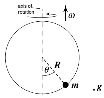
- Generalized coordinate: \(\theta\) (angle of displacement on the hoop)
-
Kinetic Energy: \(T = \frac{1}{2} m (R^2 \dot{\theta}^2 + \omega^2 R^2 \sin^2 \theta)\)
-
Potential Energy: \(V = -mgR \cos \theta\)
- Lagrangian: \(L = \frac{1}{2} m (R^2 \dot{\theta}^2 + \omega^2 R^2 \sin^2 \theta) + mgR \cos \theta\)
Applying Lagrange’s equation:
\[\frac{d}{dt} \left( \frac{\partial L}{\partial \dot{\theta}} \right) - \frac{\partial L}{\partial \theta} = 0\] \[mR^2 \ddot{\theta} - m R^2 \omega^2 \sin \theta \cos \theta + mgR \sin \theta = 0\]which governs the motion of the bead on the rotating hoop.
Hamilton’s Principle and Calculus of Variations
📘 1. Introduction to Hamilton’s Principle
Hamilton’s principle is a reformulation of classical mechanics that provides a powerful and elegant approach to deriving the equations of motion. It is also known as the principle of stationary action.
🔹 Statement of Hamilton’s Principle
The actual path taken by a physical system between two configurations at fixed times \(t_1\) and \(t_2\) is such that the action integral is stationary (usually a minimum).
Mathematically, \(\delta S = 0, \quad \text{where} \quad S = \int_{t_1}^{t_2} L(q_i, \dot{q}_i, t) \, dt\)
- \(L\) is the Lagrangian: \(L = T - V\)
- \(S\) is called the action
- \(\delta S = 0\) implies a stationary value (not necessarily minimum)
📘 2. Techniques of the Calculus of Variations
The calculus of variations deals with finding functions that make a functional stationary.
🔹 2.1 Functional Form
A functional is an integral of the form: \(J[y] = \int_{x_1}^{x_2} f(y, y', x)\, dx\) The goal is to find the function \(y(x)\) such that \(J[y]\) is stationary.
🔹 2.2 Euler-Lagrange Equation (Core Result)
If \(y(x)\) gives an extremum to \(J[y]\), then it must satisfy: \(\frac{d}{dx} \left( \frac{\partial f}{\partial y'} \right) - \frac{\partial f}{\partial y} = 0\)
🧠 Example 1: Shortest Path Between Two Points
Let’s find the shortest path between two points \(A(x_1, y_1)\) and \(B(x_2, y_2)\).
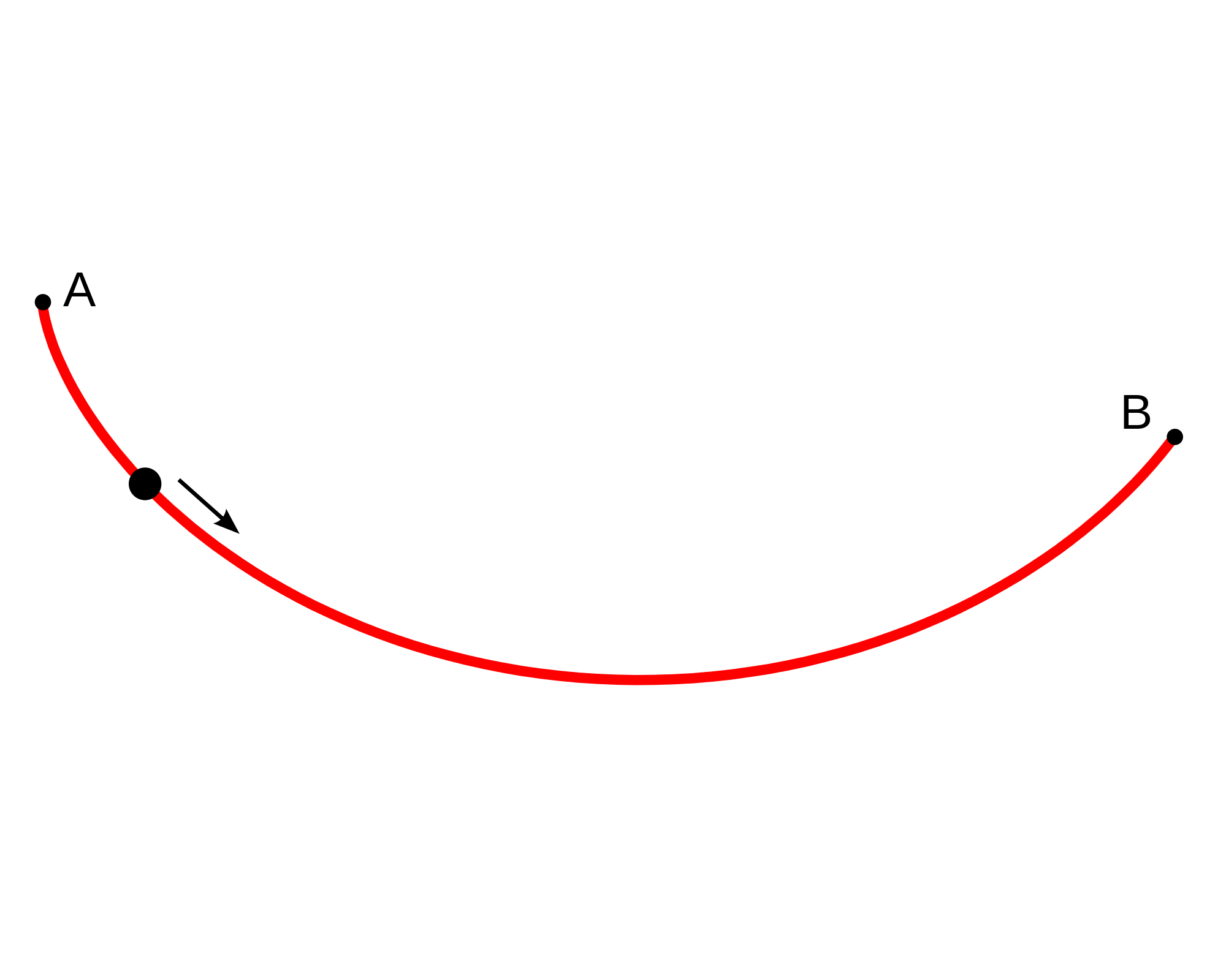
Functional: \(J[y] = \int_{x_1}^{x_2} \sqrt{1 + (y')^2} \, dx\)
Apply Euler-Lagrange:
Let \(f = \sqrt{1 + (y')^2}\), then: \(\frac{\partial f}{\partial y} = 0,\quad \frac{\partial f}{\partial y'} = \frac{y'}{\sqrt{1 + (y')^2}}\)
Now, \(\frac{d}{dx} \left( \frac{y'}{\sqrt{1 + (y')^2}} \right) = 0 \Rightarrow \frac{y'}{\sqrt{1 + (y')^2}} = C \Rightarrow y' = \text{constant} \Rightarrow y = mx + c\)
✅ The result is a straight line — confirming that the shortest path is a straight line.
📘 3. Deriving Lagrange’s Equation Using Hamilton’s Principle
🔹 3.1 Setup
Let the system have \(n\) generalized coordinates \(q_1, q_2, ..., q_n\). The Lagrangian is \(L(q_i, \dot{q}_i, t)\).
The action is: \(S = \int_{t_1}^{t_2} L(q_i, \dot{q}_i, t) \, dt\)
We vary the path \(q_i(t) \to q_i(t) + \delta q_i(t)\) with fixed endpoints: \(\delta q_i(t_1) = \delta q_i(t_2) = 0\)
We compute the variation: \(\delta S = \int_{t_1}^{t_2} \left( \sum_i \frac{\partial L}{\partial q_i} \delta q_i + \frac{\partial L}{\partial \dot{q}_i} \delta \dot{q}_i \right) dt\)
Using \(\delta \dot{q}_i = \frac{d}{dt}(\delta q_i)\), and integration by parts:
\[\int_{t_1}^{t_2} \frac{\partial L}{\partial \dot{q}_i} \frac{d}{dt}(\delta q_i) \, dt = \left. \frac{\partial L}{\partial \dot{q}_i} \delta q_i \right|_{t_1}^{t_2} - \int_{t_1}^{t_2} \frac{d}{dt} \left( \frac{\partial L}{\partial \dot{q}_i} \right) \delta q_i \, dt\]Since \(\delta q_i(t_1) = \delta q_i(t_2) = 0\), the boundary term vanishes.
Thus: \(\delta S = \int_{t_1}^{t_2} \sum_i \left( \frac{\partial L}{\partial q_i} - \frac{d}{dt} \left( \frac{\partial L}{\partial \dot{q}_i} \right) \right) \delta q_i \, dt\)
Since \(\delta q_i\) are arbitrary, for \(\delta S = 0\), the integrand must vanish:
✅ Final Result: Lagrange’s Equations
\(\frac{d}{dt} \left( \frac{\partial L}{\partial \dot{q}_i} \right) - \frac{\partial L}{\partial q_i} = 0, \quad i = 1, 2, \dots, n\)
Conservation Theorems, Symmetry, Hamilton’s Equations, and Least Action Principle
📘 1. Conservation Theorems and Symmetry Properties
In Lagrangian and Hamiltonian mechanics, symmetries of a system lead to corresponding conservation laws.
This deep connection is formally stated in Noether’s theorem.
🔹 1.1 Noether’s Theorem (Statement)
If the Lagrangian is invariant under a continuous transformation, there exists a corresponding conserved quantity.
🔹 1.2 Common Symmetries and Conservation Laws
| Symmetry Type | Conserved Quantity |
|---|---|
| Time translation invariance | Energy |
| Spatial translation | Linear momentum |
| Rotational invariance | Angular momentum |
🧠 Example: Particle in Central Force Field
Let a particle move under a central potential \(V(r)\).
- Lagrangian: \(L = \frac{1}{2} m (\dot{r}^2 + r^2 \dot{\theta}^2) - V(r)\)
- \(\theta\) is cyclic: \(\partial L / \partial \theta = 0\)
- ⇒ Angular momentum \(p_\theta = \frac{\partial L}{\partial \dot{\theta}} = m r^2 \dot{\theta}\) is conserved
📘 2. Hamilton’s Equations of Motion
Hamiltonian formulation is an alternative to Lagrangian mechanics and is especially useful in advanced physics.
🔹 2.1 Definition of the Hamiltonian
For a system with Lagrangian \(L(q_i, \dot{q}_i, t)\), define the generalized momenta: \(p_i = \frac{\partial L}{\partial \dot{q}_i}\)
Then the Hamiltonian is: \(H(q_i, p_i, t) = \sum_i p_i \dot{q}_i - L\)
🔹 2.2 Hamilton’s Canonical Equations
From the total differential \(dH\), we get:
\[\boxed{ \begin{aligned} \dot{q}_i &= \frac{\partial H}{\partial p_i} \\ \dot{p}_i &= -\frac{\partial H}{\partial q_i} \end{aligned} }\]These are Hamilton’s equations of motion.
🧠 Example: Simple Harmonic Oscillator
Lagrangian: \(L = \frac{1}{2} m \dot{x}^2 - \frac{1}{2} k x^2\)
Generalized momentum: \(p = \frac{\partial L}{\partial \dot{x}} = m \dot{x} \Rightarrow \dot{x} = \frac{p}{m}\)
Hamiltonian: \(H = p \dot{x} - L = \frac{p^2}{2m} + \frac{1}{2} k x^2\)
Hamilton’s equations: \(\dot{x} = \frac{\partial H}{\partial p} = \frac{p}{m}, \quad \dot{p} = -\frac{\partial H}{\partial x} = -k x\)
⇒ Same equations as from Newton’s second law.
📘 3. Principle of Least Action
🔹 3.1 What is Action?
Action is defined as: \(S = \int_{t_1}^{t_2} L(q_i, \dot{q}_i, t) \, dt\)
🔹 3.2 Principle of Least Action
The path taken by the system between two points in configuration space is the one that minimizes (or makes stationary) the action \(S\).
This principle is equivalent to Hamilton’s principle: \(\delta S = 0\)
It leads directly to the Euler-Lagrange equations, i.e., Lagrange’s equations: \(\frac{d}{dt} \left( \frac{\partial L}{\partial \dot{q}_i} \right) - \frac{\partial L}{\partial q_i} = 0\)
🧠 Example: Free Particle in One Dimension
- Lagrangian: \(L = \frac{1}{2} m \dot{x}^2\)
- Action: \(S = \int_{t_1}^{t_2} \frac{1}{2} m \dot{x}^2 \, dt\)
Using the calculus of variations, the path that minimizes \(S\) satisfies: \(\frac{d}{dt} \left( m \dot{x} \right) = 0 \Rightarrow \ddot{x} = 0 \Rightarrow x(t) = At + B\)
✅ The path is a straight line — consistent with Newton’s first law.
📘 4. Take Home Message
| Concept | Key Idea |
|---|---|
| Noether’s Theorem | Symmetries ⇒ Conservation laws |
| Hamilton’s Equations | 1st-order equations in \(q_i, p_i\); derived from Hamiltonian |
| Principle of Least Action | System follows path that makes action stationary |
🔍 Difference between Hamilton’s Principle and Principle of Least Action
| Aspect | Hamilton’s Principle | Principle of Least Action |
|---|---|---|
| 🔹 Definition | States that the action integral is stationary (δS = 0) | States that action is minimized (least possible S) |
| 🔹 Type of extremum | Can be minimum, maximum, or saddle point | Specifically implies a minimum |
| 🔹 Generality | More general – applies even when action is not minimum | Special case of Hamilton’s principle |
| 🔹 Mathematical Formulation | \(\delta S = 0\) | \(S = \min \int L \, dt\) |
| 🔹 Physical Use | Used to derive Lagrange’s equations | Used primarily in heuristic arguments |
✅ Note: In most practical physical systems, the action is minimized, so the two are often used interchangeably. However, Hamilton’s principle is more general.
Hamilton–Jacobi Equation
🔹 1. Introduction to Hamilton–Jacobi Theory
Hamilton–Jacobi theory provides a powerful analytical method for solving mechanical problems. It reformulates classical mechanics into a first-order partial differential equation (PDE).
🔹 2. The Hamilton–Jacobi Equation
Given a Hamiltonian \(H(q_i, p_i, t)\), the Hamilton–Jacobi equation (HJE) is:
\[\boxed{ H \left(q_i, \frac{\partial S}{\partial q_i}, t \right) + \frac{\partial S}{\partial t} = 0 }\]Here, \(S(q_i, \alpha_i, t)\) is called Hamilton’s principal function, and \(\alpha_i\) are constants of integration.
For time-independent Hamiltonians, we use Hamilton’s characteristic function \(W(q_i, \alpha_i)\):
\[\boxed{ H \left(q_i, \frac{\partial W}{\partial q_i} \right) = E }\]🔹 3. Why Use HJE?
- Converts the problem of solving \(2n\) ODEs to solving one PDE.
- Particularly useful for systems with cyclic coordinates.
- A bridge to quantum mechanics (via Schrödinger equation).
🧠 4. Example: 1D Harmonic Oscillator
Given: Mass \(m\), spring constant \(k\), natural frequency \(\omega = \sqrt{k/m}\)
Hamiltonian: \(H = \frac{p^2}{2m} + \frac{1}{2} k q^2\)
🔹 Step 1: Setup the Hamilton–Jacobi Equation
Let \(S(q, t)\) be Hamilton’s principal function.
The HJE becomes: \(\frac{1}{2m} \left( \frac{\partial S}{\partial q} \right)^2 + \frac{1}{2} k q^2 + \frac{\partial S}{\partial t} = 0\)
🔹 Step 2: Separation of Variables
Assume: \(S(q, t) = W(q) - Et\)
Substitute into HJE: \(\frac{1}{2m} \left( \frac{dW}{dq} \right)^2 + \frac{1}{2} k q^2 = E\)
🔹 Step 3: Solve for \(W(q)\)
\[\left( \frac{dW}{dq} \right)^2 = 2m \left(E - \frac{1}{2} k q^2 \right) \Rightarrow \frac{dW}{dq} = \sqrt{2m \left(E - \frac{1}{2} k q^2 \right)}\]Integrating: \(W(q) = \int \sqrt{2m \left(E - \frac{1}{2} k q^2 \right)} \, dq\)
This is a standard integral: \(W(q) = \frac{m \omega}{2} \left( q \sqrt{A^2 - q^2} + A^2 \sin^{-1}\left( \frac{q}{A} \right) \right), \quad \text{where } A = \sqrt{\frac{2E}{k}}\)
🔹 Step 4: Use Action-Angle Variables
Define the action: \(J = \oint p \, dq = \oint \sqrt{2m \left(E - \frac{1}{2} k q^2 \right)} \, dq = 2\pi \frac{E}{\omega} \Rightarrow E = \omega J\)
This leads to quantization in old quantum theory and gives the energy in terms of the action variable.
📘 Canonical Transformations and Poisson Brackets
🔹 1. Canonical Transformations
A canonical transformation is a change of phase space coordinates: \((q_i, p_i) \rightarrow (Q_i, P_i)\) that preserves the form of Hamilton’s equations.
🔸 Motivation:
Canonical transformations simplify problems by preserving the structure of Hamilton’s mechanics, particularly the symplectic structure.
symplectic structure: ensures that Hamilton’s equations remain invariant under canonical transformations and that the phase space volume is conserved over time (Liouville’s theorem).
In short, the symplectic structure guarantees that Hamiltonian dynamics are area-preserving, reversible, and fully determined by the geometry of phase space.
🔸 Condition:
The transformation is canonical if:
\[\sum_i p_i \, dq_i - H \, dt = \sum_i P_i \, dQ_i - K \, dt + dF\]where \(F\) is a generating function and \(K\) is the new Hamiltonian.
🔹 2. Generating Functions
Canonical transformations can be generated using a generating function \(F\), which can be expressed in four common types:
| Type | Generating Function | Transformation Relations |
|---|---|---|
| \(F_1(q, Q, t)\) | \(F_1\) | \(p = \partial F_1 / \partial q\), \(P = -\partial F_1 / \partial Q\) |
| \(F_2(q, P, t)\) | \(F_2\) | \(p = \partial F_2 / \partial q\), \(Q = \partial F_2 / \partial P\) |
| \(F_3(p, Q, t)\) | \(F_3\) | \(q = -\partial F_3 / \partial p\), \(P = -\partial F_3 / \partial Q\) |
| \(F_4(p, P, t)\) | \(F_4\) | \(q = -\partial F_4 / \partial p\), \(Q = \partial F_4 / \partial P\) |
✅ These functions allow us to generate transformations that maintain canonical structure.
🔹 3. Infinitesimal Canonical Transformations
An infinitesimal canonical transformation is a small transformation parameterized by \(\epsilon\):
\[Q_i = q_i + \epsilon \frac{\partial G}{\partial p_i}, \quad P_i = p_i - \epsilon \frac{\partial G}{\partial q_i}\]where \(G(q, p)\) is the generator of the transformation.
These generators are crucial in understanding symmetries and conserved quantities (via Noether’s theorem).
🔹 4. Poisson Brackets
The Poisson bracket between two functions \(f(q, p, t)\) and \(g(q, p, t)\) is defined as:
\[\{f, g\} = \sum_i \left( \frac{\partial f}{\partial q_i} \frac{\partial g}{\partial p_i} - \frac{\partial f}{\partial p_i} \frac{\partial g}{\partial q_i} \right)\]🔸 Properties:
- Antisymmetry: \(\{f, g\} = -\{g, f\}\)
- Linearity: \(\{af + bg, h\} = a\{f, h\} + b\{g, h\}\)
- Leibniz Rule: \(\{fg, h\} = f\{g, h\} + g\{f, h\}\)
- Jacobi Identity: \(\{f, \{g, h\}\} + \{g, \{h, f\}\} + \{h, \{f, g\}\} = 0\)
🔹 5. Fundamental Poisson Brackets
\[\{q_i, q_j\} = 0, \quad \{p_i, p_j\} = 0, \quad \{q_i, p_j\} = \delta_{ij}\]These relations mirror the canonical commutation relations in quantum mechanics.
🔹 6. Poisson’s Theorems
Let \(f(q, p, t)\) and \(g(q, p, t)\) be any two functions in phase space:
🔸 Theorem 1: Time Evolution
\(\frac{df}{dt} = \{f, H\} + \frac{\partial f}{\partial t}\)
This is the classical version of Heisenberg’s equation of motion.
🔸 Theorem 2: Invariance under Canonical Transformation
Poisson brackets are invariant under canonical transformations: \(\{f, g\}_{(q, p)} = \{f, g\}_{(Q, P)}\)
This invariance confirms that canonical transformations preserve physical laws.
🧠 Example: Angular Momentum Components
For a particle in 3D space, angular momentum \(\vec{L} = \vec{r} \times \vec{p}\). The components obey:
\[\{L_x, L_y\} = L_z, \quad \{L_y, L_z\} = L_x, \quad \{L_z, L_x\} = L_y\]This shows that angular momentum components generate rotational transformations.
📎 References
- H. Goldstein, Classical Mechanics, 3rd Edition
- L.D. Landau & E.M. Lifshitz, Mechanics
- V.I. Arnold, Mathematical Methods of Classical Mechanics