D’Alembert’s Principle, Lagrange’s Equation and Its Simple Applications

1. D’Alembert’s Principle

D’Alembert’s principle is a fundamental concept in classical mechanics that provides an alternative formulation of Newton’s second law by incorporating the concept of virtual work. It states that the sum of the differences between the applied forces and the inertial forces (also called the generalized forces) acting on a system in equilibrium is zero when projected along any virtual displacement.

1.1 Mathematical Formulation

Consider a system of \(N\) particles, where each particle has mass \(m_i\), position vector \(\mathbf{r}_i\), and is subject to an external force \(\mathbf{F}_i\). Newton’s second law states:

\[m_i \ddot{\mathbf{r}}_i = \mathbf{F}_i\]

D’Alembert’s principle introduces the concept of inertial force:

\[\mathbf{F}_i - m_i \ddot{\mathbf{r}}_i = 0\]

For an infinitesimal virtual displacement \(\delta \mathbf{r}_i\), the principle states:

\[\sum_{i=1}^{N} (\mathbf{F}_i - m_i \ddot{\mathbf{r}}_i) \cdot \delta \mathbf{r}_i = 0\]

Since the constraint forces do no virtual work (ideal constraints), we are left with only generalized forces:

\[\sum_{i=1}^{N} (\mathbf{F}_i^{(a)} - m_i \ddot{\mathbf{r}}_i) \cdot \delta \mathbf{r}_i = 0\]

where \(\mathbf{F}_i^{(a)}\) represents the applied forces excluding constraint forces.

2. Lagrange’s Equation

Lagrange’s equation is derived using D’Alembert’s principle and is particularly useful in dealing with systems having constraints.

2.1 Generalized Coordinates

A system with \(N\) particles and \(k\) constraint equations can be described using a reduced set of generalized coordinates:

\[q_1, q_2, \dots, q_n, \quad n = 3N - k\]

The relationship between Cartesian coordinates and generalized coordinates is given by:

\[\mathbf{r}_i = \mathbf{r}_i(q_1, q_2, ..., q_n, t)\]

The virtual displacement then transforms as:

\[\delta \mathbf{r}_i = \sum_{j=1}^{n} \frac{\partial \mathbf{r}_i}{\partial q_j} \delta q_j\]

Using these transformations, D’Alembert’s principle can be rewritten in terms of generalized coordinates.

2.2 Derivation of Lagrange’s Equation

3. Simple Applications of Lagrange’s Equations

3.1 Simple Pendulum

A simple pendulum consists of a mass \(m\) attached to a string of length \(l\). The generalized coordinate is the angular displacement \(\theta\).

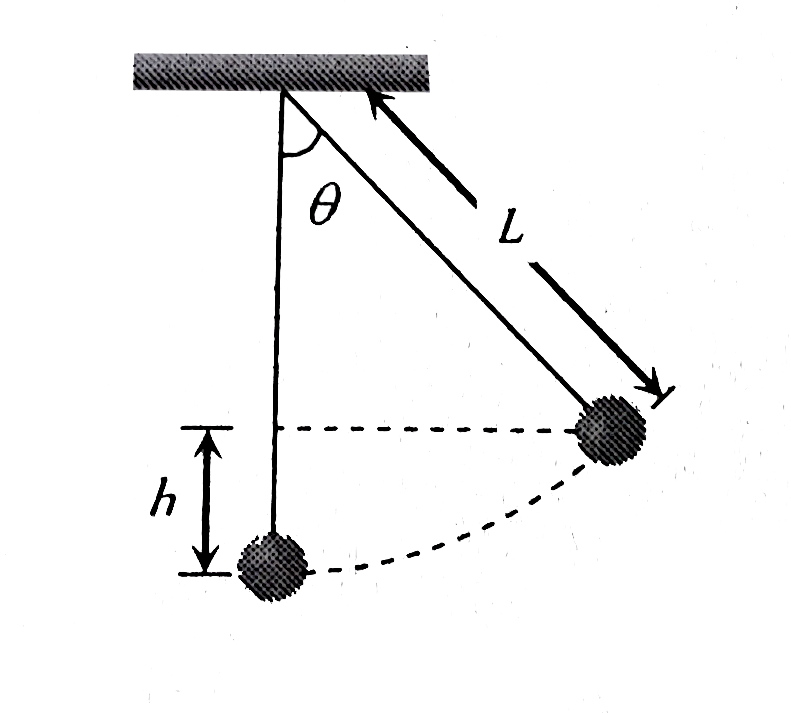
🔹 Coordinates

Use angle \(\theta\) as generalized coordinate.

• Position: \(x = \ell \sin \theta, \quad y = -\ell \cos \theta\)
• Velocity: \(v^2 = \ell^2 \dot{\theta}^2\)

🔹 Energy

• Kinetic Energy: \(T = \frac{1}{2} m (l^2 \dot{\theta}^2)\)

• Potential Energy: \(V = -mgl \cos \theta\)

🔹 Lagrangian

\[L = T - V = \frac{1}{2} m \ell^2 \dot{\theta}^2 - m g \ell (1 - \cos \theta)\]

Apply Lagrange’s equation:

\[\frac{d}{dt} \left( \frac{\partial L}{\partial \dot{\theta}} \right) - \frac{\partial L}{\partial \theta} = 0\] \[\Rightarrow \frac{d}{dt} (m \ell^2 \dot{\theta}) + m g \ell \sin \theta = 0 \Rightarrow \boxed{ \ddot{\theta} + \frac{g}{\ell} \sin \theta = 0 }\]

3.2 Bead on a Rotating Hoop

A bead of mass \(m\) moves on a hoop of radius \(R\) that rotates with a constant angular velocity \(\omega\).

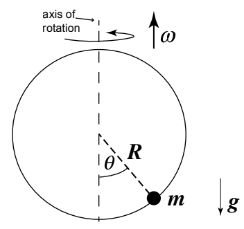
• Generalized coordinate: \(\theta\) (angle of displacement on the hoop)

• Kinetic Energy: \(T = \frac{1}{2} m (R^2 \dot{\theta}^2 + \omega^2 R^2 \sin^2 \theta)\)

• Potential Energy: \(V = -mgR \cos \theta\)

• Lagrangian: \(L = \frac{1}{2} m (R^2 \dot{\theta}^2 + \omega^2 R^2 \sin^2 \theta) + mgR \cos \theta\)

Applying Lagrange’s equation:

\[\frac{d}{dt} \left( \frac{\partial L}{\partial \dot{\theta}} \right) - \frac{\partial L}{\partial \theta} = 0\] \[mR^2 \ddot{\theta} - m R^2 \omega^2 \sin \theta \cos \theta + mgR \sin \theta = 0\]

which governs the motion of the bead on the rotating hoop.